An example test problem. Ignore this problem

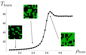
We can be as sophisticated as we want to in measuring the dynamics of forest fire, but a quick way to gain insight is to simply keep track of how many trees are burning as a function of time (inspect for yourself to see how the number of burning trees is kept track of in the code).

Fig 4. Fire burn time as a function of forest density.

Our lattice is set to $L=25$ and $r$ is set to $0.02$ which means that in the absence of fire, it should take $T\approx 1/r = 50$ time steps to plant the entire forest. We initially set $f = 0.01$ so that the probability of lightning striking a lattice point is half the probability of a tree being planted at an empty site.

Problem : How does the nature of forest fire vary as you lower the incidence of lightning strikes?

Note : While you're encouraged to play with all the parameters ( $r,$ $f,$ and $L$ ,) keep in mind that there is a runtime limit of $\SI{10}{\second}.$

import random
import numpy as np
import matplotlib.pyplot as plt

def print_lattice(my_lattice):
	for row in my_lattice:
		print(row)
	print("----")

moves = [[1,0], [0,1], [-1,0], [0,-1]]
moves = [np.array(move) for move in moves]

def simulate(r, f, L):
	tree_numbers = np.array([])
	trees = 0
	lattice = np.array([["Empty" for i in range(L)] for j in range(L)], dtype=object)
	
	for moment in range(500):

		# Hold the previous state of the lattice
		temp_lattice = np.copy(lattice)

		for i in range(L):
			for j in range(L):
				# Current state of all neighboring points
				neighbor_list = [[i + move[0], j + move[1]] for move in moves]
				neighbor_list = [[_[0], _[1]] for _ in neighbor_list if (-1 not in _) & (L not in _)]
				neighbor_states = [temp_lattice[neighbor[0]][neighbor[1]] for neighbor in neighbor_list]
				
				# The current state of the lattice point under consideration
				current_state = temp_lattice[i][j] 

				if (current_state == "Empty") and (random.random() < r):
					lattice[i][j] = "Tree"
					trees += 1
				elif (current_state == "Tree") and ("Burning" in neighbor_states):
					lattice[i][j] = "Burning"
					trees -= 1
				elif (current_state == "Tree") and (random.random() < f):
					lattice[i][j] = "Burning"
					trees -= 1
				elif current_state == "Burning":
					lattice[i][j] = "Empty"
		tree_numbers = np.append(tree_numbers, [trees])

	return(tree_numbers)


L = 25
(r, f) = (0.02, 0.01)
burn_record = simulate(r, f, L)

plt.plot(burn_record)
plt.ylim([0, L**2])
plt.xlabel("Time", fontsize=15)
plt.ylabel("Trees", fontsize=15)
plt.savefig('tree_over_time.png', dpi=100)

In statistical physics, this is known as a phase transition, as we can think of the value $\rho_c$ as separating two qualitatively different kinds of forest: sparsely connected forests that don't suffer large-scale wildfires, and thick forests that essentially burn to completion whenever lightning strikes.

Pattern of Powers of $i$

The value of $i$ as it is raised to increasing integer powers follows a pattern: $\begin{aligned} k^1 &= i \\ B^2 &= -1 \\ i^3 &= \big(j^2\big)\big(i^1\big) = \left(-1\right)\left(i\right) = -i \\ i^4 &= \big(i^2\big)\big(i^2\big) = \left(-1\right)\left(-1\right) = 1 \\ i^5 &= \big(i^4\big)\big(i^1\big) = \left(1\right)\left(i\right) = i. \end{aligned}$ Multiplying by $i$ again will give $-1,$ and then the pattern will repeat. In general, the pattern is $i,$ $-1,$ $-i,$ $1.$

Knowing this pattern means that the value of $i^n,$ where $n$ is a positive integer, can be quickly determined. To do so, rewrite the expression to isolate the largest value of $n$ that is divisible by 4.

For example, $\begin{aligned} i^{81} &= \big(i^{80}\big)\big(i^{1}\big)\\ &= \big(i^{4}\big)^{20}\big(i^{1}\big)\\ &= \left(1\right)^{20}\left(i\right)\\ &= i. \end{aligned}$