Archer duel

Why code? The cumulative standard normal distribution is a good approximation.

With a 50 shots, the number of hits of each player may be approximated by a normal distribution with $\mu = 50\alpha,\ \ \ \sigma^2 = 50\alpha(1-\alpha).$ To determine who wins, we subtract Ashleys's number of hits from Chamath's number of hits. Thus we study the random variable $X = C - A$ , which is approximately normally distributed with parameters $\mu_X = \mu_C - \mu_A = 50\cdot 0.5 - 50\cdot 0.4 = 25 - 20 = 5; \\ \sigma_X^2 = \sigma_C^2 + \sigma_A^2 = 50\cdot 0.5\cdot 0.5 + 50\cdot 0.4\cdot 0.6 = 12\tfrac12 + 12 = 24\tfrac12.$ At first, one may think that Ashley is the winner iff $X < 0$ ; however, we must account for the possibility of a tie, which in our continuous approximation would correspond to $-\tfrac12 < X < \tfrac12$ . Therefore we calculate $\mathbb P(X < -\tfrac12) = \Phi\left(\frac{\tfrac12 - 5}{\sqrt{24\tfrac12}}\right) = \Phi(-1.1112) = 0.1332.$ Here, $\Phi$ is the cumulative probability distribution (probability function) of the standard normal distribution.

This answer, $13.32\%$ is not exact due to the normal approximation of the binomial distribution, but close enough.

Okay, let's do some coding

We must calculate $\sum_{0 \leq k < j \leq N} \binom N j (1-\alpha)^{N-j} \alpha^j \binom N k (1-\beta)^{N-k} \beta^k,$ which may be written as $\sum_{i=0}^N \binom N i (1-\alpha)^{N-i} \alpha^i C_{i-1}\ \ \ \ \ \text{with}\ \ \ \ \ \ C_{i-1} = \sum_{k=0}^{i-1} \binom N k (1-\beta)^{N-k} \beta^k.$ Here is how.

Note that we only use a single loop. In this loop,

• binom = $\binom N i$ .

• powA = $(1-\alpha)^{N-j} \alpha^j$ and powC = $(1-\beta)^{N-i} \beta^i$ .

• pA and pC = probabilities that Ashley/Chamath have $i$ hits.

• cumC = $C_{i-1}$ = probability that Chamath has fewer than $i$ hits.

 1
 2
 3
 4
 5
 6
 7
 8
 9
10
11
12
13
14
15
16
17
18
19
20
21
22
23
24
25
26
27
28
29
30
31
32

#include<stdio.h>

#define MOVES 50
#define ACC_A 0.40
#define ACC_C 0.50

int main() {
    double pAwin = 0;
    double pA, pC, cumC = 0.0;

    double binom = 1, powA = 1, powC = 1;

    for (int i = 0; i < MOVES; i++) {
        powA *= (1.0 - ACC_A);
        powC *= (1.0 - ACC_C);
    }

    for (int i = 0; i <= MOVES; i++) {
        pA = binom * powA;
        pC = binom * powC;

        pAwin += pA * cumC;
        cumC += pC;

        if (i < MOVES) {
            binom *= (MOVES - i); binom /= (i+1);
            powA *= ACC_A/(1.0 - ACC_A); powC *= ACC_C/(1.0 - ACC_C);
        }
    }

    printf("%8.3f%%\n",100*pAwin);
}

Yesterday, in school, a good friend of mine asked me to help her with solving this exact problem where total number of hits was 2. Solution was pretty straightforward. Win for A would mean one of the following results $(1,0), (2,0)$ or $(2,1)$ . The final probability is the sum of the probabilities of these results: $P\left(\text{Ashley wins}\right) = \binom{2}{1}\cdot0.4^{1}\cdot0.6^{1}\cdot\binom{2}{0}\cdot0.5^{2} + \binom{2}{2}\cdot0.4^{2}\cdot\binom{2}{0}\cdot0.5^{2} + \binom{2}{2}\cdot0.4^2\cdot\binom{2}{1}\cdot0.5^2 = 0.24$ Yet, I was still left wondering if I can generalize my solution and evaluate the same probability for number of shootings greater than 2, for any $n$ , so, while I was walking back home, I gave some thought to it. The first thing I realized I had to do was to somehow categorize all winning results in an efficient way that will enable me to calculate and sum their probabilities. I began by classifying the winning results according to the difference $(d)$ between Ashley's and Chamath's accurate hits. If number of Ashley's accurate hits is denoted with $a$ and Chamath's with $c$ , it follows that:

• $1 \leq d \leq n$ ;
• $d \leq a \leq n$ ;
• $c = a - d$ .

Now, notice how each possible winning result is defined. Probability of result $(a, c)$ out of $n$ hits is: $\binom{n}{a}p^{a}(1-p)^{n-a}\binom{n}{c}q^{c}(1-q)^{n-c},$ where $p$ and $q$ are accuracies of Ashley and Chamath, respectively. We can now evaluate the final probability: $P\left(\text{Ashley wins}\right) = \sum_{d = 1}^{n}\sum_{a = d}^{n}\binom{n}{a}p^{a}(1-p)^{n-a}\binom{n}{a-d}q^{a-d}(1-q)^{n-a+d}.$ Unfortunately, from here, expression cannot be substantially simplified, so I wrote a simple function in Python to carry out calculations:

 1
 2
 3
 4
 5
 6
 7
 8
 9
10
11
12
13
14

import numpy as np
import scipy
from scipy import special
import matplotlib.pyplot as plt

def f(N, p, q):
    sum = np.zeros((len(N)))
    for i in range(len(N)):
        sum[i] = 0
        n = N[i]
        for d in range(1, n+1):
            for a in range(d, n+1):
                sum[i] += scipy.special.binom(n,a)*np.power(p, a)*np.power(1-p, n-a)*scipy.special.binom(n, a-d)*np.power(q, a-d)*np.power(1-q, n-a+d)
    return sum

Input :

1
2

prob = f([50], p, q)
print("Probability equals: %f" % prob)

Output :

1

Probability equals: 0.133353

That's desired solution, but it would be interesting to see how the probability varies relative to $n$ .

 1
 2
 3
 4
 5
 6
 7
 8
 9
10
11
12

N = np.arange(1,100,1)
p = 0.4
q = 0.5
P = f(N, p, q)
print("Maximum probability equals %f for n = %0.0f" % (max(P),np.argmax(P)+1)) #indexing in python start from 0
plt.plot(N, P)

plt.xlabel('total number of hits')
plt.ylabel('Probability that Ashley wins')
plt.title('P = %0.3f, q = %0.3f' % (p,q))
plt.savefig("plot1.png")
plt.show()

Here's the graph I got: 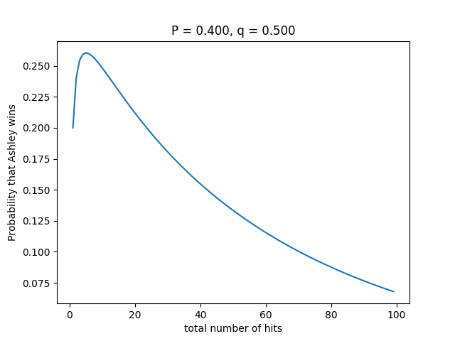It turns out that the peak of graph (maximum probability) occurs at $n = 5$ and it equals $0.26042$ .

Actually, it's also fun to alter values of $p$ and $q$ and examine corresponding graphs. Here's another one, for $p = 0.3$ and $q = 0.3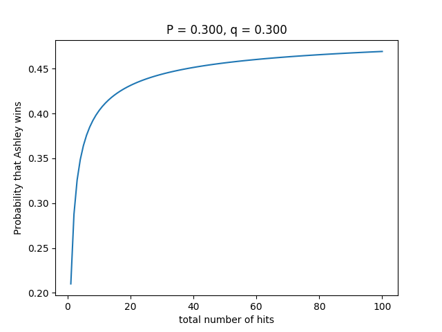$ : We can see that the probability slowly tends to $0.5$ as $n$ goes to $\infty$ . No matter how big or small accuracies are, as long as they are equal, this will be true. That's somewhat intuitive because as the number of total hits rises, it is more and more unlikely that they both had the same number of accurate hits resulting in a draw. Feel free to copy my code and paste it to your coding environment and explore the behavior of the function with other values of $p$ and $q$ .