Band Stop Filter Charging Transient

An R L C RLC band stop filter takes a sinusoidal voltage input V S ( t ) V_S(t) and produces an output voltage V o u t ( t ) V_{out} (t) .

V S ( t ) V_S(t) is as follows:

V S ( t ) = 10 sin ( t ) V_S(t) = 10 \sin(t)

At time t = 0 t = 0 , the inductor and capacitor are de-energized. Determine the following integral:

0 15 π V o u t ( t ) d t \int_0^{15 \pi} V_{out} (t) \, dt

Details and Assumptions:
1) R = 3 R = 3
2) L = 1 L = 1
3) C = 1 C = 1

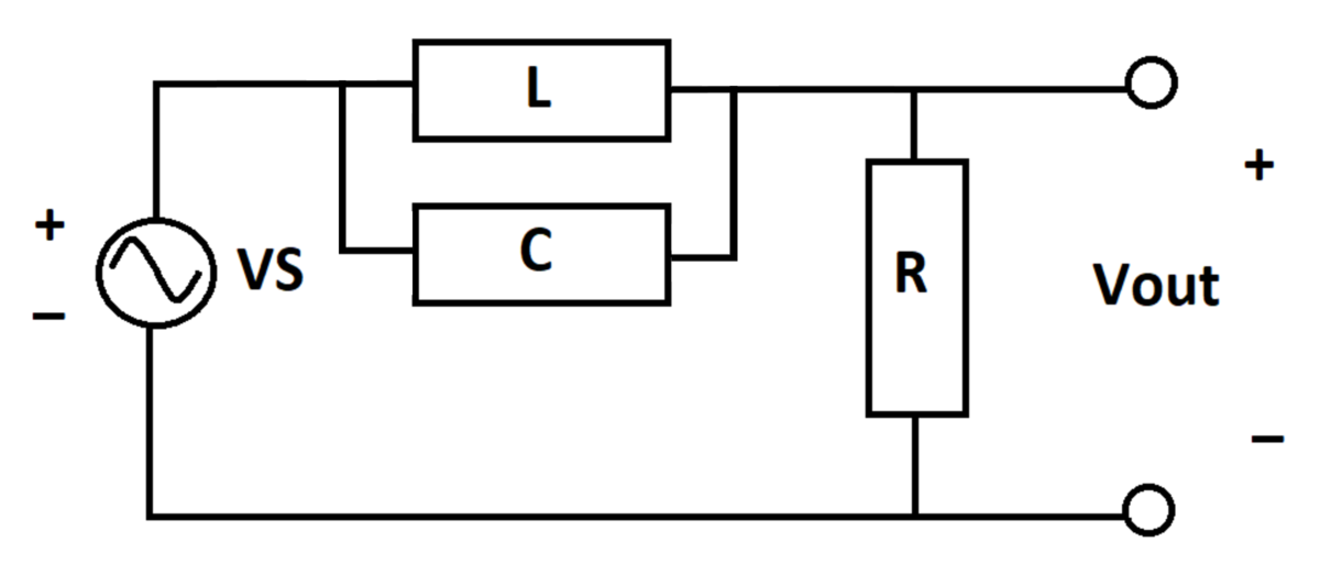
Note: From AC steady-state analysis, we know that sinusoidal signals with angular frequency ω = 1 \omega = 1 are completely rejected by this filter, once the filter has "charged up"


The answer is 10.0.

This section requires Javascript.
You are seeing this because something didn't load right. We suggest you, (a) try refreshing the page, (b) enabling javascript if it is disabled on your browser and, finally, (c) loading the non-javascript version of this page . We're sorry about the hassle.

1 solution

Karan Chatrath
Dec 15, 2019

Let the current through the inductor be I 1 I_1 and that through the capacitor be I 2 I_2 , the charge on the capacitor be Q Q and output voltage be V V . The circuit equations are:

V S + L I ˙ 1 + ( I 1 + I 2 ) R = 0 -V_S + L\dot{I}_1 + (I_1+I_2)R=0 L I ˙ 1 = Q C L\dot{I}_1=\frac{Q}{C} V = ( I 1 + I 2 ) R V= (I_1+I_2)R I 1 ( 0 ) = I 2 ( 0 ) = Q ( 0 ) = 0 I_1(0) = I_2(0) = Q(0) = 0

Numerically integrating the above equations gives the required answer of 10.002 \approx\boxed{10.002} .


I am pasting my solution to the frequency domain problem without revealing the answer below:

The circuit has been analysed in steady-state. Let the magnitude of input voltage be V V and its frequency be ω \omega . The impedance due to the inductor is Z 1 = j ω L Z_1=j\omega L and that due to the capacitor is Z 2 = 1 j ω C Z_2=\frac{-1}{j\omega C} . Let the steady-state current through the inductor be I 1 I_1 and that through the capacitor be I 2 I_2 . The circuit equations are according to Kirchoff's laws as follows.

Z 1 I 1 + ( I 1 + I 2 ) R = V Z_1I_1 + (I_1 + I_2)R = V Z 1 I 1 = Z 2 I 2 Z_1I_1 = Z_2I_2

Rearranging these equations gives:

[ Z 1 + R R Z 1 Z 2 ] [ I 1 I 2 ] = [ V 0 ] \left[\begin{matrix}Z_1+R&R\\Z_1&-Z_2\end{matrix}\right]\left[\begin{matrix}I_1\\I_2\end{matrix}\right]=\left[\begin{matrix}V\\0\end{matrix}\right]

From here, the currents can be computed as such:

[ I 1 I 2 ] = [ Z 1 + R R Z 1 Z 2 ] 1 [ V 0 ] \left[\begin{matrix}I_1\\I_2\end{matrix}\right]=\left[\begin{matrix}Z_1+R&R\\Z_1&-Z_2\end{matrix}\right]^{-1}\left[\begin{matrix}V\\0\end{matrix}\right]

The matrix is denoted as A where: A = [ Z 1 + R R Z 1 Z 2 ] A = \left[\begin{matrix}Z_1+R&R\\Z_1&-Z_2\end{matrix}\right]

The output voltage is: V o = R ( I 1 + I 2 ) V_o = R(I_1 + I_2)

The filter gain is, therefore, the ratio of the magnitude of the complex numbers:

G ( ω ) = V o V G(\omega)= \left\lvert \frac{V_o}{V} \right\rvert

Now, keeping these steps in mind, the=is problem is solved numerically. A plot of the magnitude response can be studied below:

One can see a sharp drop in magnitude ratio at a frequency of ω = 1 \omega = 1 . This can be verified by a time-domain simulation where the output voltage indeed converges to zero.

For the computation of the required integral, simulation code is attached below:

 1
 2
 3
 4
 5
 6
 7
 8
 9
10
11
12
13
14
15
16
17
18
19
20
21
22
23
24
25
26
27
28
29
30
31
32
33
34
35
36
37
38
39
40
41
42
43
44
clear all
clc

% Initialisation:
R = 3;
L = 1;
C = 1;

% Frequency range definition:
dw = 1e-4;
w  = dw:dw:5;
N  = length(w);

% Initial value of required integral:
S  = 0;

% Frequency ranges from dw (instead of zero) to 5 rad/sec in steps of dw to prevent any singularities.

% Here, j = sqrt(-1)..

for k = 1:length(w)

    % Computing the matrix A:
    Z1 = j*w(k)*L;
    Z2 = -j/(w(k)*C);
    A  = [Z1+R R;Z1 -Z2];

    % Computing the current column matrix and assuming that the amplitude of input voltage is unity:
    I  = inv(A)*[1;0];

    % Computation of output voltage magnitude which is also the Magnitude ratio in this case:
    G(k) = abs(R*(I(1)+I(2)));

    % Numerical integration of the required function:
    f  = 1 - G(k);
    S  = S + dw*f;
end

% Plotting frequency response:
plot(w,G,'Linewidth',1.5)
grid on
xlabel('Frequency [rad/sec]')
ylabel('G(\omega)')
title('Frequency Response - Magnitude Response')

Thanks for the detailed solutions to this problem set. I kind of had fun seeing the correspondence between the frequency domain and time domain results.

Steven Chase - 1 year, 5 months ago

Log in to reply

Ya, so did I. In fact, the time domain analysis validated my result for the frequency domain problem. Thanks for posting

Karan Chatrath - 1 year, 5 months ago

0 pending reports

×

Problem Loading...

Note Loading...

Set Loading...