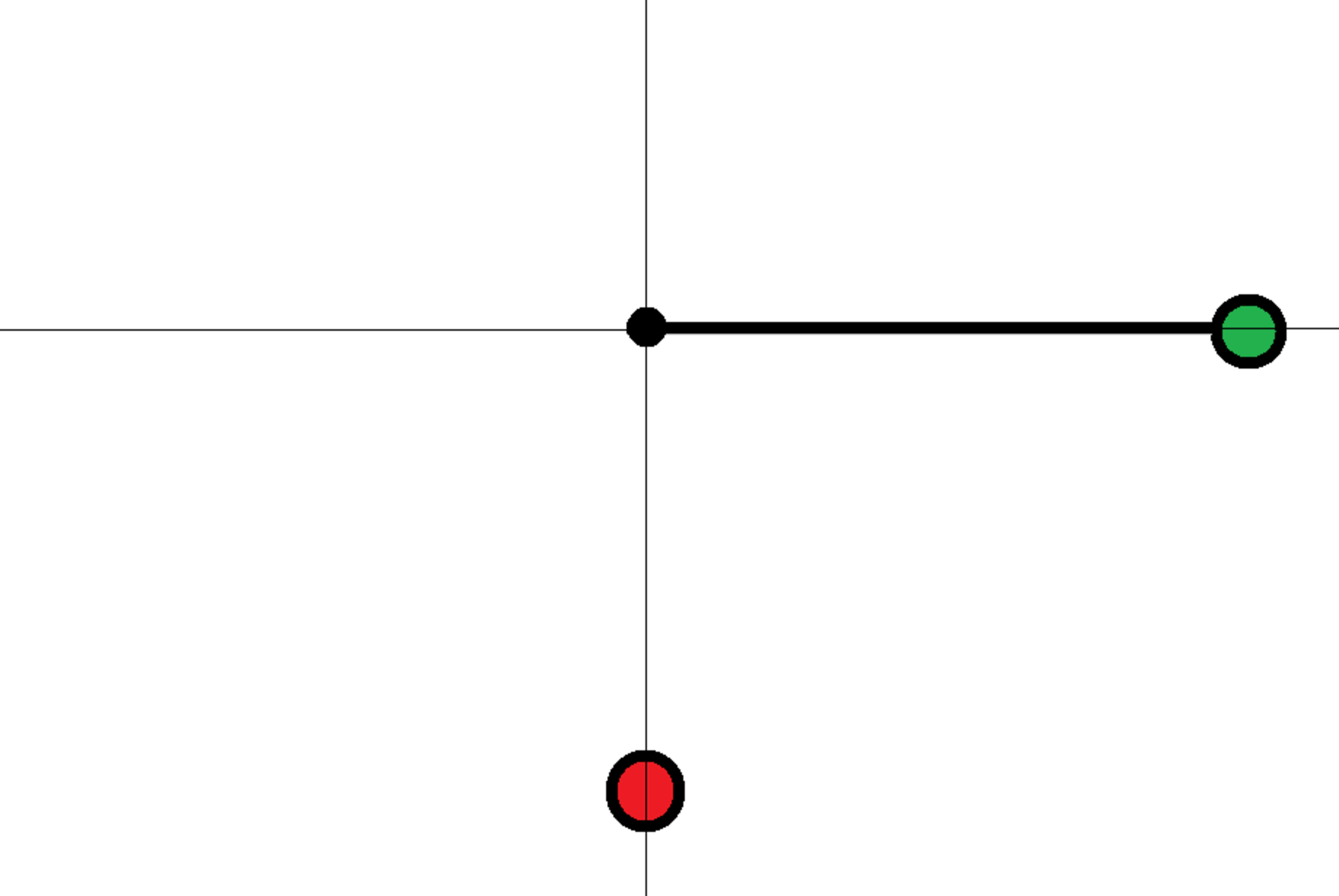
Charge Seesaw 3

This problem, just like the previous ones can be easily solved using the method of equipotential points. This time, it is apparent that the rod oscillates between $\theta=0$ and $\theta = 180^{\circ}$ . However, I have taken a deliberate numerical approach to demonstrate a partial non explicit computation of Lagrange's equations of motion:

Consider the rod to be at an angle $\theta$ at a general time $t$ . The position vector is:

$\vec{r} = (\cos{\theta},\sin{\theta})$ $\implies \vec{v} = (-\dot{\theta}\sin{\theta},\dot{\theta}\cos{\theta})$ $\vec{r}_p = (0,-1)$

Potential energy:

$V = \frac{kq^2}{\lvert \vec{r} - \vec{r}_p \rvert}$

Kinetic energy:

$T = \frac{m}{2}\lvert \vec{v} \rvert^2 = \frac{\dot{\theta}^2}{2}$

Lagrange's equation is:

$\frac{d}{dt} \left(\frac{\partial T}{\partial \dot{\theta}}\right) + \frac{\partial V}{\partial \theta}=0$ $\implies \ddot{\theta} = -\frac{\partial V}{\partial \theta}$

The derivative for potential energy is not computed explicitly, but rather numerically. I tried doing the same for kinetic energy, but I ran into numerical issues. I will attempt to resolve those in due course of time. Code attached below. From a plot of $\theta$ vs. Time, one can conclude that the time period of motion is approximately $14.3 \ \mathrm{s}$ . One can also see that $0 \le \theta \le \pi$

 1
 2
 3
 4
 5
 6
 7
 8
 9
10
11
12
13
14
15
16
17
18
19
20
21
22
23
24
25
26
27
28
29
30
31
32
33
34
35
36
37
38
39
40
41
42
43
44
45
46
47
48
49
50
51

clear all
clc

% Parameters:
K = 1;
q = 1;
m = 1;

% Initial Conditions:
theta(1)  = 0;
dtheta(1) = 0;

% Time and time step:
dt        = 1e-4;
tf        = 20;
t         = 0:dt:tf;

for k = 1:length(t)-1

    % Potential energy derivative with respect to theta:
    dV          = jacobian(theta(k),@(theta)PE(K,q,theta));

    % Lagrange's equation of motion:
    ddtheta     = -dV;

    % Numerical Integration - Semi implicit Euler:
    dtheta(k+1) = dtheta(k) + ddtheta*dt;
    theta(k+1)  = theta(k) + dtheta(k+1)*dt;
end

plot(t,theta)
grid on

% Function for Potential Energy:
function V = PE(K,q,theta)

rp        = [0;-1;0];
r         = [cos(theta);sin(theta);0];

V         = (K*q^2)/norm(r - rp);

end

% Function for Numerical Jacobian (partial derivative):
function J = jacobian(q,f)

eps = 1e-9;

J   = (f(q + eps) - f(q))/eps;

end