Cicada 3305

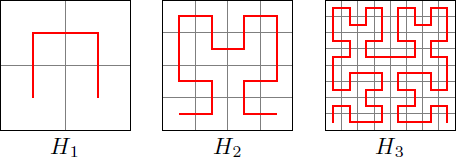
The Hilbert curve is a continuous curve that can be defined by recursion and completely fills a square in the limit $n \to \infty$ . For illustration, the first three iterations of the Hilbert curve are shown here:

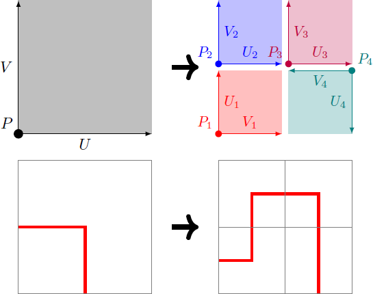
The $n$ th Hilbert curve $H_n$ is a polygonal chain with $2 ^ {2n}$ vertices, all lying on a square grid. In each iteration step, an elementary square is split into four sub-squares. The vertex of a single square is $P = (x, y)$ and there are two vectors $U = (u_x, u_y)$ and $V = (v_x, v_y)$ that span the square. The vector $U$ is the connection vector to the vertex of the following square. This square is divided into four sub-squares each having a vertex $P_i$ and the vectors $U_i$ and $V_i$ ( $i = 1,2 , 3.4$ ). This is done according to the following scheme: In algebraic form this yields $\begin{aligned} P_1 &= P, & U_1 &= \frac{1}{2} V, & V_1 &= \frac{1}{2} U \\ P_2 &= P + \frac{1}{2} V, & U_2 &= \frac{1}{2} U, & V_2 &= \frac{1}{2} V \\ P_3 &= P + \frac{1}{2} (U + V) & U_3 &= \frac{1}{2} U, & V_3 &= \frac{1}{2} V \\ P_4 &= P + U + \frac{1}{2} V & U_4 &= -\frac{1}{2} V, & V_4 &= -\frac{1}{2} U \end{aligned}$ Note, that the sum of the connection vectors $U_1 + U_2 + U_3 + U_4 = U$ returns the original vector, so that the following squares correctly connect with the previous ones. If one hangs all connection vectors one after the other, one obtains the Hilbert curve of the current iteration step.

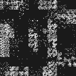
If we interpreted the underlying grid of squares as a picture with $2 ^ n \times 2 ^ n$ pixels, the Hilbert curve gives us a way to iterate over all the pixels in the image. If you then arrange these pixels line by line in the order in which they were traversed by the Hilbert curve, the result is a new image. In this way, information can be encoded and decoded.

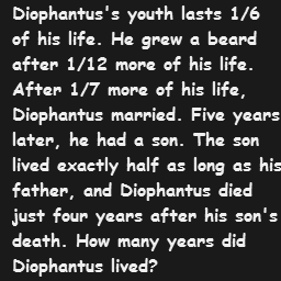
In our case, the image has $256 \times 256$ pixels, so we need the Hilbert curve $H_8$ to traverse all the pixels. The fact that the image is actually arranged in the form of a Hilbert curve can be seen in the rectangular structures. By trial and error one finds that the start and end point of the Hilbert curve lie respectively in the left and right lower corner of the image. If we transform our image according to the same scheme as above, the following text results:

This is the well-known Diophantus's riddle. Let $D$ be the age of Diophantus in years, then it follows $\begin{aligned} & & \frac{D}{6} + \frac{D}{12} + \frac{D}{7} + 5 + \frac{D}{2} + 4 &= D \\ \Rightarrow & & \frac{25}{28} D + 9 &= D \\ \Rightarrow & & 9 &= \frac{3}{28} D \\ \Rightarrow & & D &= 9 \cdot \frac{28}{3} = 84 \end{aligned}$ Thus, 84 is the correct answer.

The following Python program converts the image into readable text. The function hilbert generates the Hilbert curve according to the recursion shown above and returns a list of points connected in series giving the Hilbert curve. The vectors $P$ , $U$ and $V$ and the returned points are represented as complex numbers. The recursion automatically stops when the side length of the elemental squares is only 1.

 1
 2
 3
 4
 5
 6
 7
 8
 9
10
11
12

import numpy as np
from PIL import Image

def hilbert(P,U,V):
    if abs(U)<=1:
        return [P+U/2+V/2]
    else:
        return hilbert(P,V/2,U/2) + hilbert(P+V/2,U/2,V/2) + hilbert(P+(U+V)/2,U/2,V/2) + hilbert(P+V/2+U,-V/2,-U/2)

img = np.array(Image.open('Cicada3305.png').convert('L'))
newImg = np.array([img[int(z.real)][int(z.imag)] for z in hilbert(256j,256,-256j)], dtype='uint8')
Image.fromarray(newImg.reshape((256,256))).save('plaintext.png')