Criss Cross Loop Flux
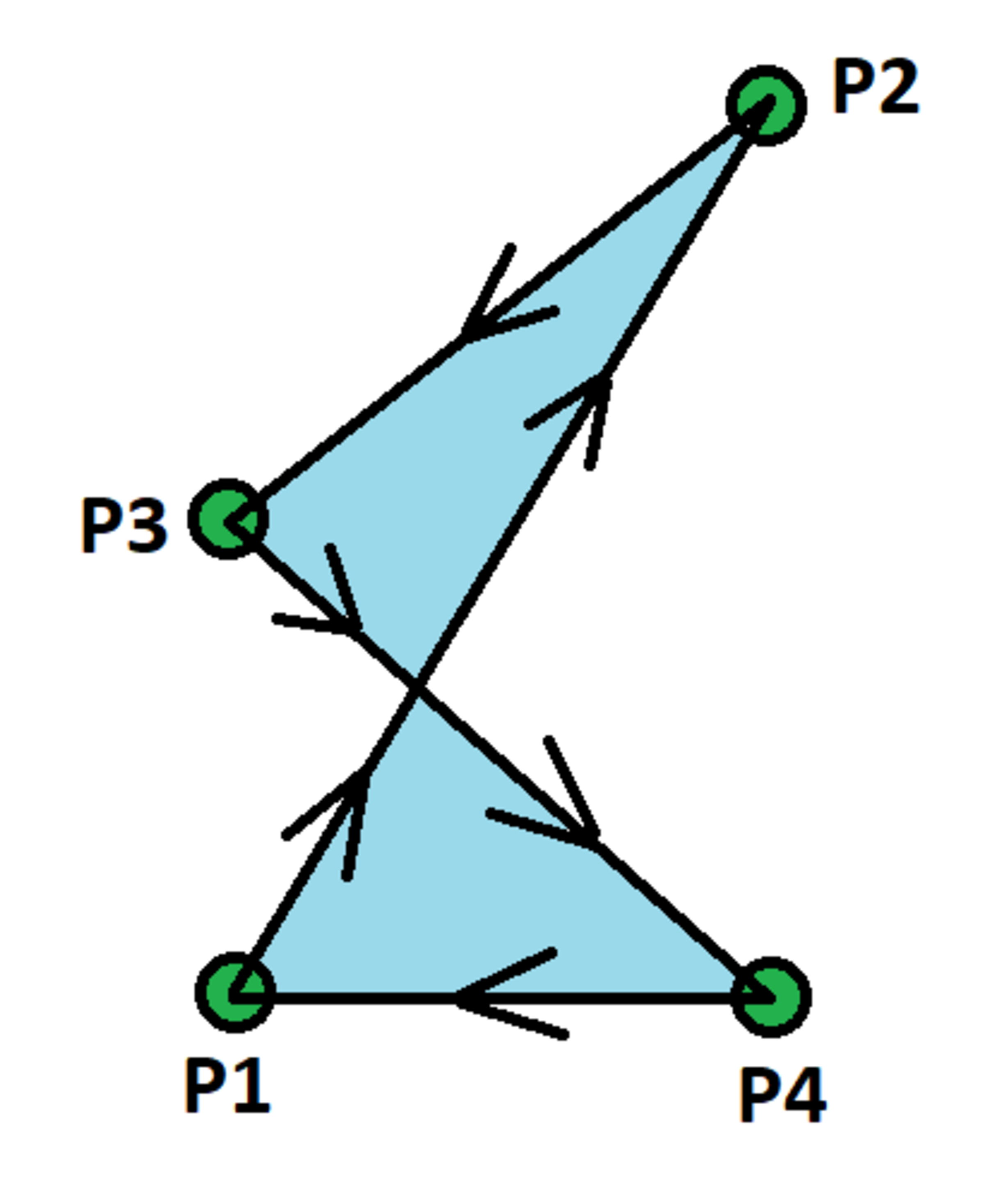
A closed loop consists of straight lines from point to point , from point to point , from point to point , and from point to point , as shown in the diagram. The point coordinates are (in format):
There is a magnetic vector potential all throughout space. The magnetic flux density is the curl of the magnetic vector potential.
Determine the absolute value of the magnetic flux through the loop:
The answer is 0.5.
This section requires Javascript.
You are seeing this because something didn't load right. We suggest you, (a) try
refreshing the page, (b) enabling javascript if it is disabled on your browser and,
finally, (c)
loading the
non-javascript version of this page
. We're sorry about the hassle.
The equation of the line connecting P1 and P2 can be parameterised as:
x = t y = 2 t z = t
t varies from 0 to 1 . We have:
A = ( 2 t , t , t ) d r = ( 1 , 2 , 1 ) d t
∫ P 1 → P 2 A ⋅ d r = ∫ 0 1 5 t d t = 2 5
The equation of the line connecting P2 and P3 can be parameterised as:
x = 1 − t y = 2 − t z = 1 − t
t varies from 0 to 1 . We have:
A = ( 2 − t , 1 − t , 1 − t ) d r = ( − 1 , − 1 , − 1 ) d t
∫ P 2 → P 3 A ⋅ d r = − ∫ 0 1 ( 4 − 3 t ) d t = − 2 5
The equation of the line connecting P3 and P4 can be parameterised as:
x = t y = 1 − t z = 0
t varies from 0 to 1 . We have:
A = ( 1 − t , 0 , t ) d r = ( 1 , − 1 , 0 ) d t
∫ P 3 → P 4 A ⋅ d r = ∫ 0 1 ( 1 − t ) d t = 2 1
The equation of the line connecting P3 and P4 can be parameterised as:
x = 1 − t y = 0 z = 0
t varies from 0 to 1 . We have:
A = ( 0 , 0 , 1 − t ) d r = ( 1 , 0 , 0 ) d t
∫ P 4 → P 1 A ⋅ d r = ∫ 0 1 0 d t = 0
Now, the flux through the closed-loop
Φ = ∫ S B ⋅ d S = ∮ C A ⋅ d r
The above identity is found using Stokes' theorem. Then:
Φ = ∮ C A ⋅ d r = ( ∫ P 1 → P 2 A ⋅ d r ) + ( ∫ P 2 → P 3 A ⋅ d r ) + ( ∫ P 3 → P 4 A ⋅ d r ) + ( ∫ P 4 → P 1 A ⋅ d r ) = 2 5 − 2 5 + 2 1 + 0 ⟹ Φ = 2 1