Damped Oscillation 12-4-2020
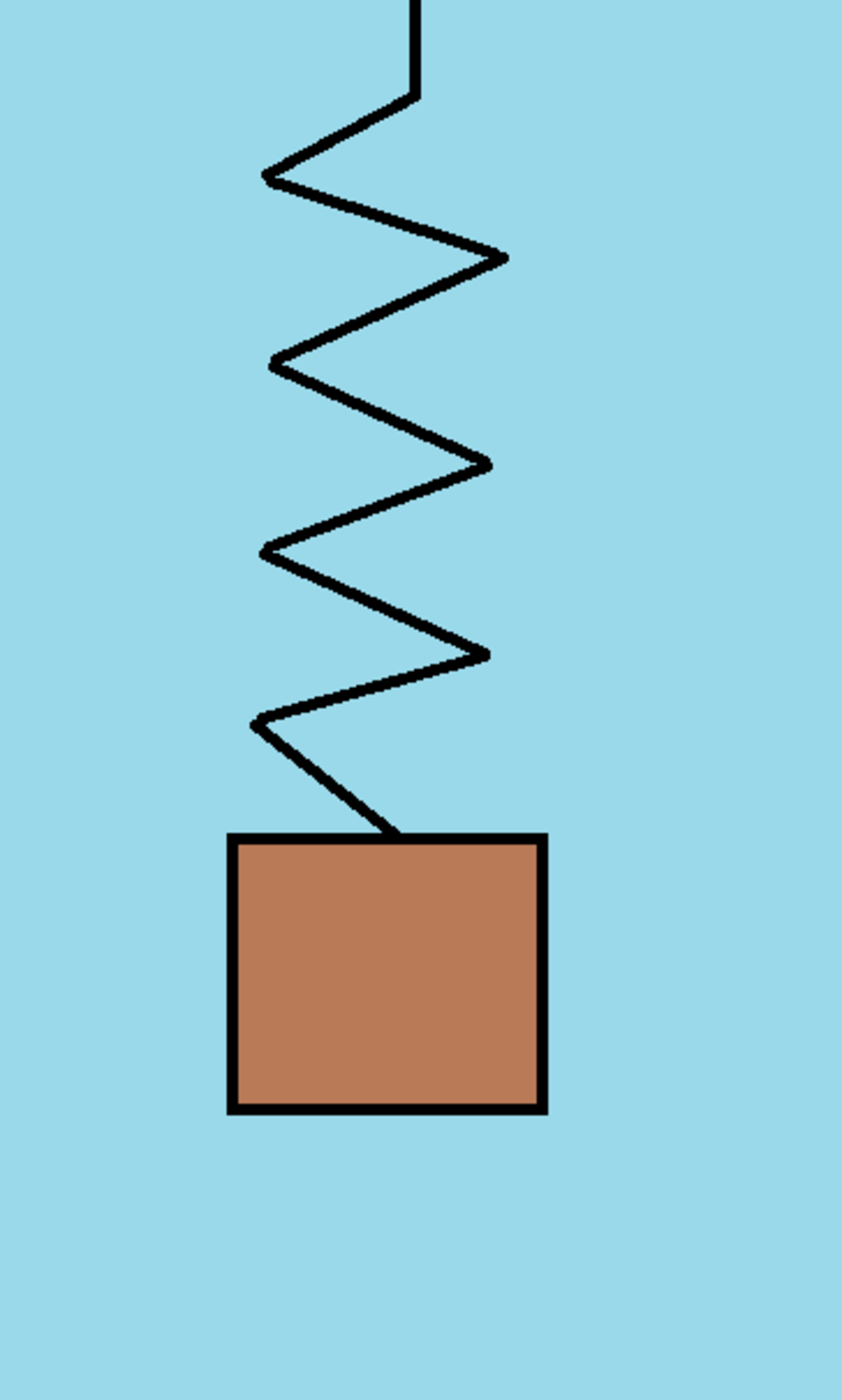
A mass m m is connected to one end of a spring of force constant k k . The other end of the spring is fixed in place. At time t = 0 t = 0 , the spring is at its natural length, and the mass is at rest at position y = 0 y = 0 . The ambient gravitational acceleration g g is downward, which corresponds to the + y +y direction. As the mass moves, it is subjected to damping forces, such that the differential equation describing its motion is:

m y ¨ = m g k y D y ˙ m \ddot{y} = m g - k y - D \dot{y}

What is the position of the mass at time t = 7 t = 7 ?

Details and Assumptions:
1) m = 1 m = 1
2) g = 10 g = 10
3) k = 5 k = 5
4) D = 0.5 D = 0.5
5) Assume standard S I SI units for all quantities


The answer is 2.337.

This section requires Javascript.
You are seeing this because something didn't load right. We suggest you, (a) try refreshing the page, (b) enabling javascript if it is disabled on your browser and, finally, (c) loading the non-javascript version of this page . We're sorry about the hassle.

2 solutions

Hosam Hajjir
Dec 4, 2020

Substituting the given parameters in the given differential equation, we obtain,

y ¨ + 0.5 y ˙ + 5 y = 10 \ddot{y} + 0.5 \dot{y} + 5 y = 10

Taking the Laplace transform of the both sides, and keeping in mind that y ( 0 ) = y ˙ ( 0 ) = 0 y(0) = \dot{y}(0) = 0 ,

s 2 Y ( s ) + 0.5 s Y ( s ) + 5 Y ( s ) = 10 s s^2 Y(s) + 0.5 s Y(s) + 5 Y(s) = \dfrac{10}{s}

So that,

Y ( s ) = 10 s ( s 2 + 0.5 s + 5 ) = 10 s ( ( s + a ) 2 + b 2 ) Y(s) = \dfrac{ 10 } { s (s^2 + 0.5 s + 5 ) } = \dfrac{ 10 }{ s ( (s + a)^2 + b^2 )}

where a = 0.25 a = 0.25 , b 2 = 5 a 2 b^2 = 5 - a^2

Using partial fractions, Y ( s ) Y(s) can be expressed as follows:

Y ( s ) = 10 s ( ( s + a ) 2 + b 2 ) = A s + B ( s + a ) ( s + a ) 2 + b 2 + C b ( s + a ) 2 + b 2 Y(s) = \dfrac{10}{ s( (s + a)^2 + b^2 ) } = \dfrac{A}{s} + \dfrac{ B (s + a) }{ (s + a)^2 + b^2 } + \dfrac{ C b } { (s + a)^2 + b^2 }

And this means that,

10 = A ( ( s + a ) 2 + b 2 ) + B s ( s + a ) + C b s 10 = A ( (s + a)^2 + b^2 ) + B s (s + a) + C b s

Equating equal powers of s s on both sides of the equation, we deduce that,

0 = A + B 0 = A + B

0 = 2 A a + B a + C b 0 = 2 A a + B a + C b

10 = A ( a 2 + b 2 ) 10 = A (a^2 + b^2)

Hence,

A = 10 a 2 + b 2 A = \dfrac{10}{a^2 + b^2}

B = 10 a 2 + b 2 B = - \dfrac{10}{a^2 + b^2}

C = a b ( 2 A + B ) = 10 a b ( a 2 + b 2 ) C = - \dfrac{a}{b} (2 A + B ) = - \dfrac{10 a}{b(a^2 + b^2)}

Finally, we Laplace invert the partial fraction expansion of Y ( s ) Y(s) , to get,

y ( t ) = A + B e a t cos ( b t ) + C e a t sin ( b t ) y(t) = A + B e^{-a t} \cos( b t ) + C e^{-at} \sin(b t )

Using the values of a , b a , b , we find that A = 2 , B = 2 , C = 0.22501758 A = 2 , B = -2 , C = -0.22501758 , hence, substituting t = 7 t = 7 , we get,

y ( 7 ) 2.337 y(7) \approx \boxed{ 2.337 }

Good use of the Laplace Transform. I for one just solved using an RK4 solver 🤣

Krishna Karthik - 6 months, 1 week ago
Krishna Karthik
Dec 5, 2020

It's been a long, long time. It's good to be back.

Here's the differential equation:

y ¨ = 10 5 y 0.5 y ˙ \ddot{y} = 10-5y-0.5 \dot{y}

Solve using RK4 till t = 7 t = 7 :

 1
 2
 3
 4
 5
 6
 7
 8
 9
10
11
12
13
14
15
16
17
18
19
20
21
22
23
24
25
26
27
28
29
30
31
32
33
34
35
36
37
38
39
40
41
42
43
44
45
46
47
48
49
#4th order Runge-Kutta numerical solution of second order ODE 

import math 

#initialisation 

def sin(x): 
    return math.sin((math.pi/180)*x) 

def cos(x): 
    return math.cos((math.pi/180)*x) 

time = 0 
deltaT = 10**-4


u_1 = 0
u_2 = 0

def differentialEquation(t,x,xdot):  #applying RK4 by splitting 2nd order ODE into 2 first order ODEs 
    return (10-5*x-0.5*xdot)


while time <= 7: 

    #evaluating slope at various points 


    k0 = deltaT*u_2 
    L0 = deltaT*differentialEquation(time,u_1,u_2) 

    k1 = deltaT*(u_2 + 0.5*L0) 
    L1 = deltaT*differentialEquation(time + 0.5*deltaT, u_1 + 0.5*k0, u_2 + 0.5*L0) 

    k2 = deltaT*(u_2 + 0.5*L1) 
    L2 = deltaT*differentialEquation(time + 0.5*deltaT, u_1 + 0.5*k1, u_2 + 0.5*L1) 

    k3 = deltaT*(u_2 + L2) 
    L3 = deltaT*differentialEquation(time + deltaT, u_1 + k2, u_2 + L2) 


    #RK4 approximation of values 

    u_1 = u_1 + (1/6)*(k0 + 2*k1 + 2*k2 + k3) 
    u_2 = u_2 + (1/6)*(L0 + 2*L1 + 2*L2 + L3) 

    time += deltaT 

print(u_1)

0 pending reports

×

Problem Loading...

Note Loading...

Set Loading...