Death defying skateboard stall
Skateboarder Bob Burnquist has big ramps in his backyard that he's always trying to do bigger and better things with. Recently, Bob had a
helicopter pilot hover over his quarterpipe
so that he could air and stall on the helicopter's skids.
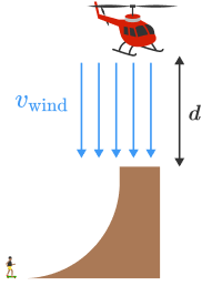
Due to gravity alone Bob has to go pretty fast to air out of the quarterpipe at all but the helicopter provides a massive downward thrust that requires Bob to go even faster. This is a terrifying experience because as you approach the ramp you feel like you have enough speed to air through the blades.
The crucial factor that prevents this is that the air being pushed through the blades works to decelerate Bob's ascent. We can model the drag force on Bob as F d = 2 1 ρ c d A v relative 2 , where v relative = v wind + v Bob .
Find Bob's speed at the top of the ramp (in m / s ) such that he comes to rest exactly at the height of the skids, d = 4 m above the ramp.
You may want to use the code environment below.
Assume : v wind = 3 0 m / s is the steady windspeed of the air coming down through the blades, Bob's cross sectional area is A = 1 . 3 2 m 2 , the drag coefficient for the human body is c d = 1 , ρ = 1 . 2 2 k g / m 3 , g = 1 0 m / s 2 , and m Bob = 9 0 k g .
import matplotlib.pyplot as plt

g = 10
v_wind = 30
m_bob = 90
C = 0.5 * 1.22 * 1.32

time = 0
height = 0
velocity = 1 # <- You'll want to experiment with this initial value.

(times, heights) = ([], []) # <- Arrays to collect the values of height and time.

# Write code to propagate height and velocity forward in time and
# collect them in the lists, times and heights.


# Uncomment this code to plot h as a function of time.
# plt.plot(times, heights)
# plt.title('$h_\mathrm{max}$ is %f m' % heights[-1])
# plt.xlabel('Time ($t$)')
# plt.ylabel('$h_\mathrm{max}$')
# plt.savefig("my_plot.png")
The answer is 13.7285.
This section requires Javascript.
You are seeing this because something didn't load right. We suggest you, (a) try
refreshing the page, (b) enabling javascript if it is disabled on your browser and,
finally, (c)
loading the
non-javascript version of this page
. We're sorry about the hassle.
4 solutions
Total KE required at highest point = energy needed to overcome drag due to wind + energy needed to escape gravitational pull. KE = dragforce × distance + mgh ; 1/2mV^2 = 1/2×density×Cd×(30+V)^2×4 + mgh ; 0.5×90×V^2 = 0.5×1.22×1×(30+V)^2 ×4 + 90×10×4. Solving above equation gives the required answer:))
Log in to reply
Because the speed changes during the jump, so does the drag force. Therefore the work cannot be calculated using W = F Δ y directly, but must be obtained by integration, W = ∫ F d y ; or, equivalently, you need a differential equation approach, d W = F d y . No matter how you go about it, this problem requires calculus or numerical simulation/integration.
Log in to reply
Is he correct about the energy equation he has shown?
There is a typo: κ = 2 m ρ C d A at the top.
Dear me, what complications! If you write the acceleration as v.dv/ds (s being distance) you then get a straightforward integration by separating the variables, giving implicit equation: (b^2)/20.ln(((u+30)^2 + b^2)/(900 + b^2)) - 3b.arc tan(ub/(b^2 + 900 + 30u)) = 4, where u = take-off velocity and b^2 = 900/0.8052. By successive approximation this gives u = 13.73924757 (to about 8 insignificant figures, in view of the data) I give all these digits only because I do not agree with 13.7285, the answer you give.
Log in to reply
Your equation is equivalent to my equation for λ t just above the horizontal line. It is indeed not necessary to work with dimensionless quantities as I did, but I find that it gives some additional insight in the problem. Your approach of writing a = d t d v = d t d s d s d v = v d s d v is a nice shortcut for the integration.
Log in to reply
Wow, this can avoid time in the solution because question only gives velocity and displacement. Did the same way!
How did you go about finding the value of β 0 ?
1 2 3 4 5 6 7 8 9 10 11 12 13 14 15 16 17 18 19 20 21 22 23 24 25 26 27 28 29 30 31 32 |
|
I'm not sure this works. Here's my solution:
1 2 3 4 5 6 7 8 9 10 11 12 13 14 15 16 17 18 19 20 21 22 23 24 25 26 27 28 29 30 31 32 33 34 35 36 37 38 39 40 41 42 43 44 45 46 47 48 49 50 51 52 53 54 55 56 57 58 59 60 61 62 63 64 65 |
|
The question is written so that one might attempt to set a finite starting velocity and adjust it until velocity is zero at 4m. The other way around is much simpler and straight forward, assuming v=0 at t=0, working backward in time to what the velocity must be in order to fulfill that.
1 2 3 4 5 6 7 8 9 10 11 12 13 14 15 16 17 18 19 20 21 22 23 |
|
It's a good thing Newton's laws are symmetric with respect to time reversal.
Log in to reply
Are there any physical laws which are not time symmetric?
Log in to reply
In a way the fluctuation relations describe an asymmetry in that the probability of a process that produces entropy ω during its evolution, compared to the probability of the time reversed process (with entropy production − ω ) is given by P ( ω ) = P ( − ω ) e ω . But none of the fundamental dynamical laws (e.g. Newton's law, the Dirac equation, etc.).
1 2 3 4 5 6 7 8 9 10 11 12 13 14 15 16 17 18 19 20 21 22 23 24 25 26 27 28 29 30 31 32 33 34 35 36 |
|
Here is a more traditional solution, without using the code.
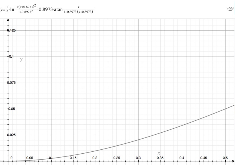
The equation of motion is d t 2 d 2 y = m − F d − F g = − κ ( d t d y + w ) 2 − g , κ = 2 m ρ C d A . Switch to dimensionless units, as follows: t ⋆ = g κ 1 = 3 . 3 4 3 s ; v ⋆ = κ g = 3 3 . 4 3 m / s ; y ∗ = κ 1 = 1 1 . 7 7 m . τ = t ⋆ t ; β = v ⋆ v ; λ = y ⋆ y . The equation of motion becomes − d τ 2 d 2 λ = ( d τ d λ + ω ) 2 + 1 , where ω = w / v ⋆ = 0 . 8 9 7 3 is the dimensionless wind speed. Setting β r e l = d λ / d τ + ω , this becomes − d τ d β r e l = β r e l 2 + 1 . Integration yields d τ d λ = β r e l − ω = tan ( τ 0 − τ ) − ω . Here, τ 0 is an integration constant. It corresponds to the time when Bob will be falling down at speed w .
We integrate again: λ = ln cos τ 0 cos ( τ 0 − τ ) − ω τ . The integration constant was chosen to ensure that λ = 0 at τ = 0 .
If Bob's initial speed (at τ = 0 ) is d λ / d τ = β 0 = v 0 / v ⋆ , then we find tan τ 0 = β 0 + ω . Bob reaches the highest points at τ = τ 0 , when d λ / d τ = 0 , so that tan ( τ 0 − τ t ) = ω . We write for the greatest height λ t = ln cos ( τ 0 − τ t ) cos τ 0 − ω τ t ; using cos x = 1 / 1 + tan 2 x and tan τ t = tan ( τ 0 − ( τ 0 − τ t ) ) , we eliminate the τ variables: λ t = 2 1 ln 1 + ω 2 1 + ( β 0 + ω ) 2 − ω inv tan 1 + ( β 0 + ω ) ω β 0 . We are told that λ t = y t / y ⋆ = 0 . 0 3 5 7 9 ; in principle, we could solve this equation for β 0 using numerical methods; we find β 0 ≈ 0 . 4 1 1 and v 0 ≈ 1 3 . 7 4 m / s .
An approximate solution may be obtained by Taylor approximations and ignoring higher powers than β 0 2 . We have λ t ≈ 2 1 [ 1 + ω 2 2 ω β 0 + ( 1 + ω 2 ) 2 ( 1 − ω ) 2 β 0 2 ] − [ 1 + ω 2 ω β 0 − ( 1 + ω 2 ) 2 ω 2 β 0 2 ] = ( 1 + ω 2 ) 2 1 − 2 ω + 3 ω 2 ⋅ 2 1 β 0 2 . Solving, we obtain β 0 ≈ 1 − 2 ω + 3 ω 2 1 + ω 2 2 λ t . (Note: β 0 = 2 λ t would be the approximation without wind and ignoring air resistance, corresponding to the familiar v 0 = 2 g h .)
In our situation, this becomes β 0 ≈ 0 . 3 7 9 3 , v 0 ≈ 1 2 . 7 m / s . The fact that β is not significantly less than unity shows that this approximation is not great. Indeed, we are 7% low-- but it gives at least an idea of the answer!