Dynamics (3-28-2020)
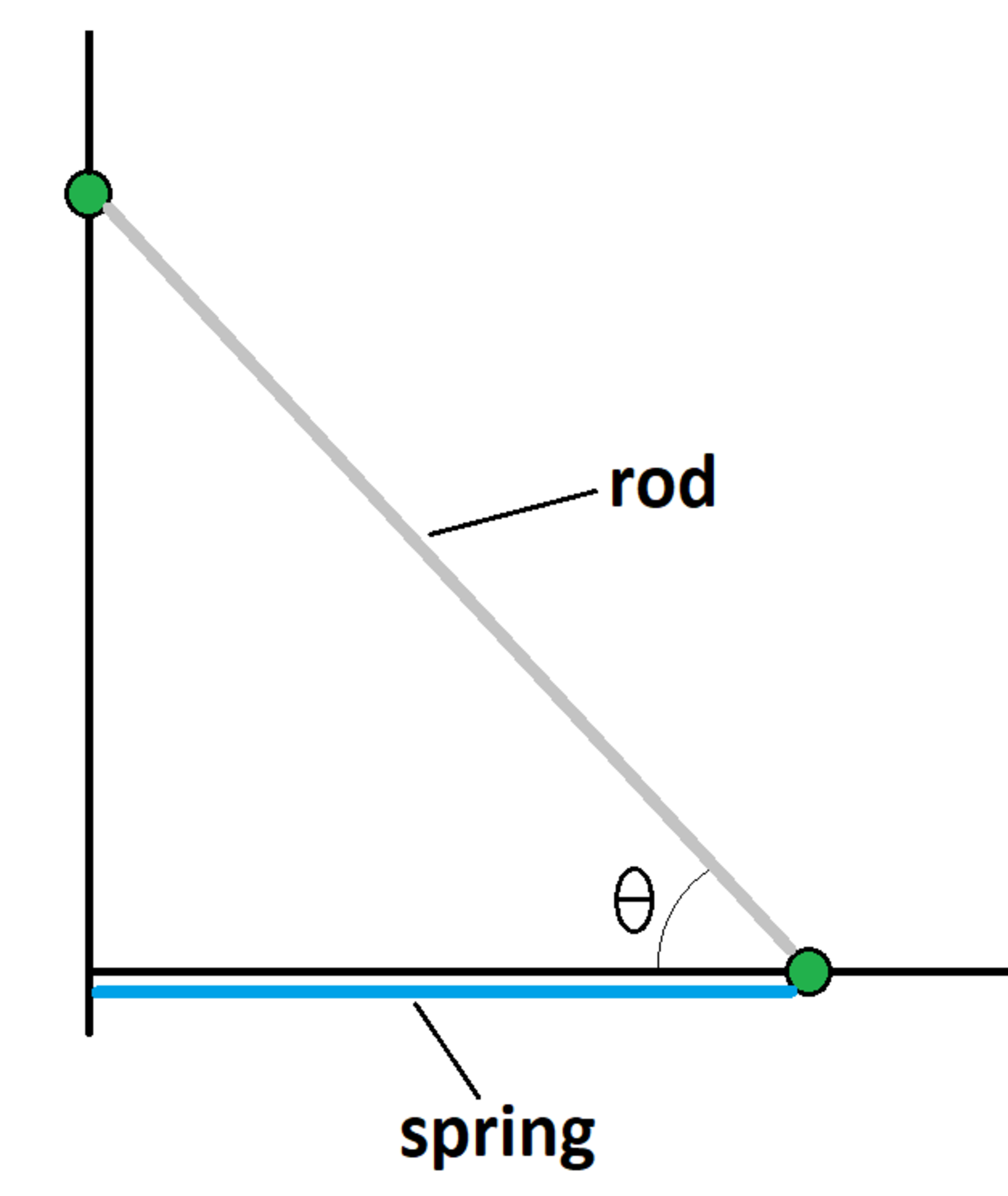
Two identical particles of mass are fixed to the and axes, respectively, where they can slide without losses. The particles are attached to the ends of a mass-less rigid rod of length , and the angle between the rod and the axis is . A spring of force constant and natural length has one end connected to the origin, and the other end connected to the particle on the axis. The ambient gravitational acceleration is in the direction.
If the system starts from rest with , what is the time period of the system's motion?
Details and Assumptions:
1)
2)
3)
4)
5)
6)
The answer is 2.068.
This section requires Javascript.
You are seeing this because something didn't load right. We suggest you, (a) try
refreshing the page, (b) enabling javascript if it is disabled on your browser and,
finally, (c)
loading the
non-javascript version of this page
. We're sorry about the hassle.
Consider the particle on the x-axis. It's coordinates are:
x 1 = L cos θ ⟹ x ˙ 1 = − L θ ˙ sin θ y 1 = 0
Consider the particle on the y-axis. It's coordinates are:
x 2 = 0 y 2 = L sin θ ⟹ y ˙ 2 = L θ ˙ cos θ
At any instant of time, the kinetic energy of the whole system of particles is:
T = 2 1 m ( x ˙ 1 2 + y ˙ 1 2 ) + 2 1 m ( x ˙ 2 2 + y ˙ 2 2 ) = θ ˙ 2
At any instant of time, the potential energy of the system is:
V = V g r a v i t a t i o n a l + V s p r i n g V = m g y 1 + m g y 2 + 2 1 k ( x 1 − L o ) 2 V = 1 0 2 sin θ + 2 9 5 ( 2 cos θ − 1 ) 2
Since the total energy of the system is conserved, by applying the law of conservation of energy, one gets:
E = T + V = T i n i t i a l + V i n i t i a l = 1 0 E = θ ˙ 2 + 1 0 2 sin θ + 2 9 5 ( 2 cos θ − 1 ) 2 = 1 0
The initial potential energy can be computed by plugging in θ = π / 4 . To obtain the equation of motion (EOM) of this system, all that needs to be done now is:
d t d E = 0
Evaluating the above expression gives the required EOM and numerical integration gives the required answer quite easily. However, I did not take this route. Here is what I tried.
The total energy of the system is conserved. If this system were to undergo periodic motion, the oscillations would take place such that θ oscillates between two extremities. One extreme position is known which is θ = π / 4 . The question then becomes to find the other extreme position. To do this, one must understand that at the other extreme position, the system would have lost all kinetic energy and would have only potential energy. Since energy is conserved, this value of the extreme potential energy is 10. To find the other extreme position, the potential energy needs to be equated to 10 and θ must be solved for. However, solving a nonlinear equation is not so trivial. So I plotted the potential energy of the system vs. θ as follows and drew the following conclusions:
Using these insights, the energy equation can be re-arranged as follows:
E = θ ˙ 2 + 1 0 2 sin θ + 2 9 5 ( 2 cos θ − 1 ) 2 = 1 0 1 0 − 1 0 2 sin θ − 2 9 5 ( 2 cos θ − 1 ) 2 = θ ˙
As time increases, θ decreases which justifies the introduction of a negative sign as such: 1 0 − 1 0 2 sin θ − 2 9 5 ( 2 cos θ − 1 ) 2 = − θ ˙
Separating the variables and integrating can give the required expression for the T time period which is:
2 T = ∫ θ m θ o 1 0 − 1 0 2 sin θ − 2 9 5 ( 2 cos θ − 1 ) 2 d θ T ≈ 2 . 0 6 6
The above integral was outsourced to Wolfram. The value of θ m was obtained to high precision as the value of the integral is sensitive to it. The answer was verified by regular brute-force numerical integration of the EOM.