Epic RLC circuit
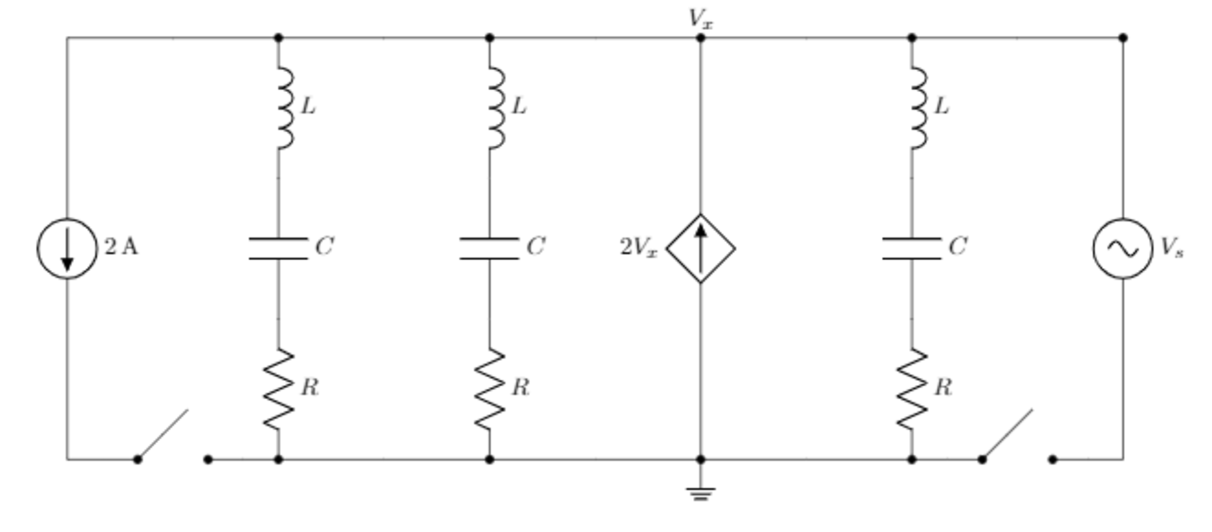
Consider the following RLC circuit which contains an AC source, a current source and a voltage controlled current source. The circuit has been in the current state for a very long time. The switches are closed simultaneously at
t
=
0
.
 If the current through the AC source is
i
(
t
)
, calculate
Q
=
∫
0
2
π
i
(
t
)
d
t
Enter your answer as
∣
Q
∣
.
If the current through the AC source is
i
(
t
)
, calculate
Q
=
∫
0
2
π
i
(
t
)
d
t
Enter your answer as
∣
Q
∣
.
Values:
- R = 7 Ω .
- C = 1 0 0 m F .
- L = 1 H .
- V s ( t ) = 0 . 2 sin ( 5 t ) V .
Inspired by Steven Chase's problem .
The answer is 12.55.
This section requires Javascript.
You are seeing this because something didn't load right. We suggest you, (a) try
refreshing the page, (b) enabling javascript if it is disabled on your browser and,
finally, (c)
loading the
non-javascript version of this page
. We're sorry about the hassle.
3 solutions
Here's a solution using Laplace-Transforms. We use the same currents and voltages Charley Shi defined in the other solution and assume V s ( t ) is defined downward. Before we begin, we normalize all currents, voltages, time and elements by the values given below: voltages: 1 V , currents: 1 A , time: 1 s ⇒ R : 1 Ω , C : 1 F , L : 1 H , Q : 1 C The network equations remain the same in the process, but now all currents, voltages, time and elements represent their normalized dimensionless counterparts.
Before switching ( t < 0 )
Assume the network is asymptotically stable for all t < 0 (discussion in the appendix)
Both input sources can be omitted, as they are only connected on one side. Assuming the remaining network is asymptotically stable, it will be in steady state for all t < 0 , because it exists for all time and has no input sources. In this steady state, all currents and voltages are zero.
After switching ( t ≥ 0 )
All initial conditions vanish at t = 0 − because of the steady state for t < 0 . We notice V x ( t ) = V s ( t ) , so we may regard the controlled source as another independent input source. We also notice by symmetry of the elements and initial conditions, we must have i 1 ( t ) = i 2 ( t ) = i 3 ( t ) .
Now we compute i ( t ) . As the initial conditions vanish, it only depends on three input sources. We use superposition and consider each input source independently. For both current sources, all impedances are shorted and can be omitted, so we directly get i ( t ) . For the remaining input V s ( t ) we need a transfer function H ( s ) :: H ( s ) = V s ( s ) I ( s ) = 3 1 ( s L + R + s C 1 ) 1 = s 2 C L + s R C + 1 s 3 C = L 3 ⋅ s 2 + s L R + C L 1 s = s 2 + 7 s + 1 0 3 s = ( s + 2 ) ( s + 5 ) 3 s For the input V s ( t ) with Laplace-Transform V s ( s ) , we use PFD by Covering-Method to split the single real poles: I ( s ) = H ( s ) V s ( s ) = ( s + 2 ) ( s + 5 ) 3 s ⋅ s 2 + 2 5 5 ⋅ 0 . 2 PFD = 3 [ 3 ⋅ 2 9 − 2 ⋅ s + 2 1 + 3 ⋅ 5 0 5 ⋅ s + 5 1 + s 2 + 2 5 X s + Y ] , X , Y ∈ R We don't need to calculate the coefficients X , Y , as that part will cancel later anyway. Via superposition of all three sources and inverse Laplace-Transform, we get i ( t ) = 2 − 2 V s ( t ) + 3 3 [ − 2 9 2 e − 2 t + 5 0 5 e − 5 t + K cos ( 5 t + φ ) ] , K , φ ∈ R Again, we don't need to calculate the actual values of amplitude K and phase φ , as that part will cancel out anyway, just like V s ( t ) of the controlled source. The reason is both functions are sines/cosines with a period of 5 2 π , and we integrate over five whole periods: Q ( 2 π ) = ∫ 0 2 π i ( t ) d t = 4 π − 0 + [ 2 9 1 e − 2 t − 5 0 1 e − 5 t ] 0 2 π + 0 = 4 π − 2 9 1 ( 1 − e − 4 π ) + 5 0 1 ( 1 − e − 1 0 π ) ≈ 1 2 . 5 5 2
Missing units and stability
Rem.: The controlled current source and V s ( t ) (not yet normalized) might be missing some units: V s ( t ) = 0 . 2 V sin ( 5 s − 1 t ) , i x ( t ) = 2 Ω − 1 V x ( t )
Rem.: Let's think about asymptotic stability for t < 0 . As the controlled current source is oriented against the voltage V x ( t ) , the resulting element equation is equivalent to a negative resistance R x = − 0 . 5 Ω : It seems highly unlikely that the resulting network could be asymptotically stable.
However, the state space model for t < 0 actually yields all six poles with negative real part, so the network is asymptotically stable despite the controlled current source. I suspect the other resistances are large enough so that they can compensate the destabilizing negative resistance of the controlled current source.
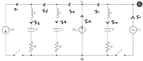
Applying Kirchoff's current law:
I = I 1 + I 2 I 3 = I X + I 1 I 3 = I 4 + I 5 I 5 = 2 + I 6
⟹ I 3 = I 4 + 2 + I 6 ⟹ I X + I 1 = I 4 + 2 + I 6 ⟹ I X + I − I 2 = = I 4 + 2 + I 6 ⟹ I = I 2 + I 4 + I 6 − I X + 2
Now, applying Kirchoff's voltage law to various loops gives:
− V S + V X = 0 ⟹ V X = V S ⟹ I X = 2 V S L I ˙ 2 + C Q 2 + I 2 R = 0 L I ˙ 4 + C Q 4 + I 4 R = 0 L I ˙ 6 + C Q 6 + I 6 R = 0 Q ˙ 2 = I 2 Q ˙ 4 = I 4 Q ˙ 6 = I 6
The initial conditions can be deciphered from the fact that at when the switches are open, no current flows and that all capacitors discharge over a long period of time. Therefore:
The current through each RLC branch is governed by:
L I ˙ b + C Q b + I b R = 0 Q ˙ b = I b Q b ( 0 ) = I b ( 0 ) = 0 b = 2 , 4 , 6
The above is solved numerically as follows:
1 2 3 4 5 6 7 8 9 10 11 12 13 14 15 16 17 18 19 20 21 22 23 24 25 26 27 28 29 30 31 32 33 34 35 36 37 38 39 40 41 42 43 44 45 46 47 48 49 50 51 |
|
Now calculate i ′ ( 0 ) . We know that i 1 ( 0 + ) = i 2 ( 0 + ) = i 3 ( 0 + ) = 0 ; this forces the voltages across all of the resistors to be zero. In addition, the capacitors have zero voltage across them immediately after the switches are closed since a capacitor's voltage cannot change instantaneously. Thus, the voltage across the inductors, which can change instantaneously, must be equal to V s . However, we know V s ( 0 ) = 0 so d t d i 1 = L V s ( 0 ) = 0 . Same goes for i 2 and i 3 .
Rearranging the KCL equation and differentiating: i = i 1 + i 2 + i 3 − 2 V s + 2 d t d i = d t d i 1 + d t d i 2 + d t d i 3 − 2 d t d V s i ′ ( 0 ) = 0 + 0 + 0 − 2 cos ( 5 ( 0 ) ) = − 2 Using node voltage V s : V s = i 1 R + L d t d i 1 + C 1 ∫ i 1 ( t ) d t V s = i 2 R + L d t d i 2 + C 1 ∫ i 2 ( t ) d t V s = i 3 R + L d t d i 3 + C 1 ∫ i 3 ( t ) d t 3 V s = R ( i 1 + i 2 + i 3 ) + L ( d t d i 1 + d t d i 2 + d t d i 3 ) + C 1 ∫ i 1 ( t ) + i 2 ( t ) + i 3 ( t ) d t 3 V s = R ( i + 2 V s − 2 ) + L d t d ( i + 2 V s − 2 ) + C 1 ∫ ( i + 2 V s − 2 ) d t Differentiating: 3 d t d V s = R d t d i + 2 R d t d V s + L d t 2 d 2 i + 2 L d t 2 d 2 V s + C 1 ( i + 2 V s − 2 ) L d t 2 d 2 i + R d t d i + C 1 i ( t ) = 3 d t d V s − 2 R d t d V s − 2 L d t 2 d 2 V s − C 2 V s + C 2 Use L = 1 H , R = 7 Ω , C = 1 0 0 m F , V s = 0 . 2 sin ( 5 t ) . d t d V s = 1 cos ( 5 t ) d t 2 d 2 V s = − 5 sin ( 5 t ) Simplify RHS: ( 3 − 2 ( 7 ) ) cos ( 5 t ) − 2 ( − 5 sin ( 5 t ) ) − 0 . 1 2 ( 0 . 2 sin ( 5 t ) ) + 0 . 1 2 = − 1 1 cos ( 5 t ) + 1 0 sin ( 5 t ) − 4 sin ( 5 t ) + 2 0 d t 2 d 2 i + 7 d t d i + 1 0 i ( t ) = 6 sin ( 5 t ) − 1 1 cos ( 5 t ) + 2 0 Use trial solution method to find solution to homogeneous version. λ 2 + 7 λ + 1 0 = ( λ + 5 ) ( λ + 2 ) = 0 λ 1 = − 5 λ 2 = − 2 i c ( t ) = A e − 5 t + B e − 2 t Guess for particular solution is i p ( t ) = a sin ( 5 t ) + b cos ( 5 t ) + c . i p ′ ( t ) = 5 a cos ( 5 t ) − 5 b sin ( 5 t ) i p ′ ′ ( t ) = − 2 5 a sin ( 5 t ) − 2 5 b cos ( 5 t ) Substitute into ODE: ( − 2 5 a sin ( 5 t ) − 2 5 b cos ( 5 t ) ) + 7 ( 5 a cos ( 5 t ) − 5 b sin ( 5 t ) ) + 1 0 ( a sin ( 5 t ) + b cos ( 5 t ) + c ) = 6 sin ( 5 t ) − 1 1 cos ( 5 t ) + 2 0 ( − 1 5 a − 3 5 b ) sin ( 5 t ) + ( 3 5 a − 1 5 b ) cos ( 5 t ) + 1 0 c = 6 sin ( 5 t ) − 1 1 cos ( 5 t ) + 2 0 Equating coefficients: − 1 5 a − 3 5 b = 6 3 5 a − 1 5 b = − 1 1 1 0 c = 2 0 ⟶ c = 2 ( − 1 5 3 5 − 3 5 − 1 5 ) ( a b ) = ( 6 − 1 1 ) 5 ( − 3 7 − 7 − 3 ) ( a b ) = ( 6 − 1 1 ) ( a b ) = 5 ( 3 2 + 7 2 ) 1 ( − 3 − 7 7 − 3 ) ( 6 − 1 1 ) = 5 ( 3 2 + 7 2 ) 1 ( − 1 8 − 7 7 − 4 2 + 3 3 ) = 5 ( 3 2 + 7 2 ) 1 ( − 9 5 − 9 ) a = 3 2 + 7 2 − 1 9 b = 5 ( 3 2 + 7 2 ) − 9 i ( t ) = A e − 5 t + B e − 2 t − 3 2 + 7 2 1 9 sin ( 5 t ) − 5 ( 3 2 + 7 2 ) 9 cos ( 5 t ) + 2 i ′ ( t ) = − 5 A e − 5 t − 2 B e − 2 t − 3 2 + 7 2 9 5 cos ( 5 t ) + 3 2 + 7 2 9 sin ( 5 t ) Use initial conditions i ( 0 ) = 2 and i ′ ( 0 ) = − 2 . 2 = A + B − 5 ( 3 2 + 7 2 ) 9 + 2 ⟶ A + B = 2 9 0 9 − 2 = − 5 A − 2 B − 3 2 + 7 2 9 5 ⟶ 5 A + 2 B = 2 − 5 8 9 5 = 5 8 2 1 ( 1 5 1 2 ) ( A B ) = ( 2 9 0 9 5 8 2 1 ) ( A B ) = − 3 1 ( 2 − 5 − 1 1 ) ( 2 9 0 9 5 8 2 1 ) = 3 − 1 ( 2 9 0 1 8 − 2 9 0 1 0 5 2 9 0 − 4 5 + 2 9 0 1 0 5 ) = 3 − 1 ( 2 9 0 − 8 7 2 9 0 6 0 ) = ( 2 9 0 2 9 2 9 0 − 2 0 ) A = 1 0 1 B = 2 9 − 2 i ( t ) = 1 0 e − 5 t − 2 9 2 e − 2 t − 5 8 1 9 sin ( 5 t ) − 2 9 0 9 cos ( 5 t ) + 2 Net amount of charge is the integral over the time interval. Q = ∫ 0 2 π 1 0 e − 5 t − 2 9 2 e − 2 t − 5 8 1 9 sin ( 5 t ) − 2 9 0 9 cos ( 5 t ) + 2 d t Integrating the sine and cosine terms on [ 0 , 2 π ] result in zero, Thus, we just have Q = ∫ 0 2 π 1 0 e − 5 t − 2 9 2 e − 2 t + 2 d t = 5 0 − e − 5 t + 2 9 e − 2 t + 2 t ∣ ∣ ∣ 0 2 π = 5 0 − e − 1 0 π + 2 9 e − 4 π + 4 π + 5 0 1 − 2 9 1 = 2 9 e − 4 π − 1 + 5 0 1 − e − 1 0 π + 4 π ≈ 1 2 . 5 5