Fault Location from Consecutive Waveform Samples
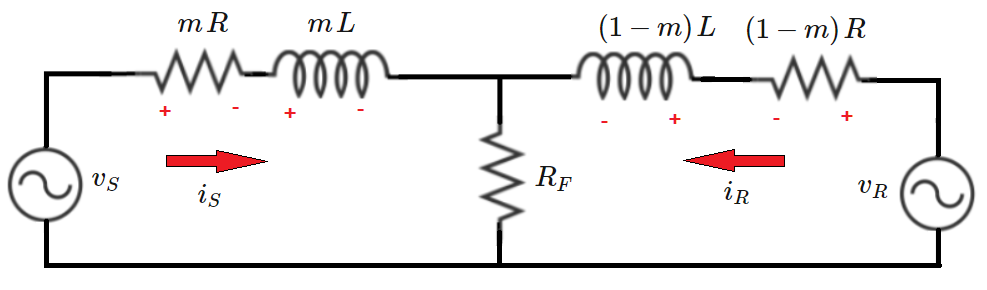
A cable is excited from both ends by ideal 6 0 Hz AC sources v S and v R . The cable has a total resistance ( R = 1 Ω ) and a total inductance ( L = 1 2 0 π 5 H ) . The resistance and inductance are distributed uniformly over the cable's length.
There is a line-to-neutral fault somewhere along the cable with unknown resistance R F . The currents flowing to the fault from the sources are i S and i R .
The following waveform samples, taken 1 0 μ s apart in time, are available (in instantaneous volts and amps):
v S ( t 0 ) = 1 5 7 . 2 5 9 4 0 0 0 4 2 v R ( t 0 ) = 1 6 8 . 0 8 6 8 7 7 7 4 8 i S ( t 0 ) = 3 6 . 5 5 7 5 5 4 6 1 8 7 i R ( t 0 ) = 5 1 . 2 4 0 7 7 6 1 8 4 2
v S ( t 0 + 1 0 − 5 ) = 1 5 7 . 0 1 7 7 9 1 1 0 9 v R ( t 0 + 1 0 − 5 ) = 1 6 8 . 1 7 3 8 3 7 8 9 8 i S ( t 0 + 1 0 − 5 ) = 3 6 . 6 4 0 9 9 2 9 5 4 1 i R ( t 0 + 1 0 − 5 ) = 5 1 . 6 0 9 2 5 1 6 7 5 9
Let the quantity m be the fractional distance to the fault, relative to the location of source v S . For example, m = 0 . 3 would correspond to a fault at a distance of 3 0 % of the cable's length away from v S .
For the particular fault under consideration, what is ( 1 0 0 m ) , to the nearest integer?
The answer is 77.
This section requires Javascript.
You are seeing this because something didn't load right. We suggest you, (a) try
refreshing the page, (b) enabling javascript if it is disabled on your browser and,
finally, (c)
loading the
non-javascript version of this page
. We're sorry about the hassle.
Express the voltage at the fault point in terms of the quantities from both sides:
v S − m R i S − m L i S ˙ = v R − ( 1 − m ) R i R − ( 1 − m ) L i R ˙
Re-arrange for an expression for the fractional fault position:
m = R i S + L i S ˙ + R i R + L i R ˙ v S − v R + R i R + L i R ˙
The only tricky part about this is the current derivative terms. That is why two sets of data are given, separated by a very short time interval relative to the signal period. The current derivative terms can be calculated by using the two sets of waveform data and taking difference quotients. Plugging in numbers yields a fault location of approximately 7 7 % .