Forest fire

Forest fires are a fact of life on a planet covered in trees. Some are minor occurrences, burning over a few acres before being snuffed out without event, while others take hold of hundreds of square miles, rage for months and destroy tremendous swaths of forest and property.

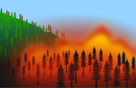
Knowing which course a wildfire will take is difficult and involves a number of factors that are hard to model, but there are fundamental questions we might expect to be insensitive to the details such as

• How long will a typical fire burn?
• What fraction of a typical forest will be destroyed?
• Are there any structural features we can exploit to reduce the severity of forest fires?

Here, we're going to build a simple model that we can interrogate in a controlled way.

1. First of all, we're going to model the forest as an $L\times L$ lattice, at each point of which a tree can exist or not.
2. Next, we're going to assume that trees are placed at lattice points with probability $\rho,$ so that the expected number of trees in the forest is $\langle \textrm{Trees}\rangle = \rho L^2.$
3. Finally, any given tree burns for one timestep, and if a tree at point $\left(i, j\right)$ is on fire at time $t,$ all nearest-neighbor trees will be on fire at time $t+1.$

We start the fire by randomly lighting one tree at time zero.

As we increase $\rho,$ the density of trees in the forest increases, as does the likelihood that trees form clusters. Therefore, we might expect that the extent and duration of the average forest fire varies as some function of $\rho.$

When $L=25,$ find $\rho_\textrm{max},$ the tree density at which the expected duration of the forest fire is maximal.

$$
Note: The code environment below has a runtime limit of $\SI{10}{\second},$ so be judicious in how you measure the forest. There are three functions in the imported module available for your use: add_lists() which takes two lists of length two and returns their vector sum, dedupe_list() which takes a list of lists and returns its unique elements, and print_forest() which takes a forest lattice and returns a pretty print representation of the state of the forest.

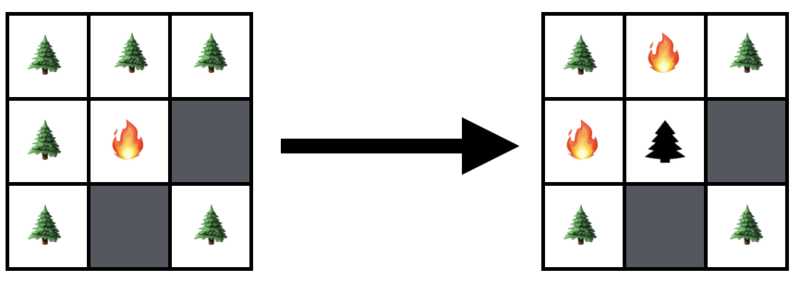
Diagram: At time $t=0,$ the tree at $\left(1,1\right)$ is lit on fire. At time $t=1$ the first tree is burned out and the fire has spread to the trees at $\left(1,0\right)$ and $\left(0,1\right)$ .

import random
import numpy as np
import matplotlib.pyplot as plt
from brilliant import forest_fire_module as fire

def simulate(p, L):
    # Initializes the lattice with a random placement of trees and a record of their status (burned or not burned)
    lattice = [[(["Tree", "NotBurned"] if random.random() < p else ["Empty", None]) 
                for i in range(L)] 
                for j in range(L)]
    
    # Possible moves for the fire to make.
    moves = [[1,0], [0,1], [-1,0], [0,-1]]
    
    # Randomly select a tree from the forest to set on fire.
    trees = [np.array([i, j]) 
                for i in range(L) 
                for j in range(L) 
                if lattice[i][j][0] is "Tree"]
    initial = random.choice(trees)
    
    # Set its status to burned in the lattice.
    lattice[initial[0]][initial[1]][1] = "Burned"
    
    # Set counters for the number of burned trees and the total
    # duration of the forest fire.
    (burn_duration, trees_burned) = (1, 1)

    # Initialize a list of all trees currently on fire.
    burning = [initial]

    print("The fire starts at", initial, "\n")
    fire.print_forest(lattice)
    
    # Fill this in with your code that propagates the fire across the forest.
    # You may find the function print_forest (used above) useful in checking your dynamics.
    # You may find the functions add_lists and dedupe_list useful as well.

    return [burn_duration, trees_burned, len(trees)]

simulate(0.4, 25)

# # Once your simulation function is working, uncomment this code and use it to measure duration
# # as a function of tree density.
# probabilities = np.arange(0.1, 1., 0.1)
# mean_burned = []
# mean_durations = []
# 
# for p in probabilities:
#   tmp_burn_durations = []
#   tmp_fractions_burned = []
#   for measurement in range(100):
#       [burn_duration, trees_burned, trees_total] = simulate(p, 25)
#       tmp_burn_durations.append(burn_duration)
#       tmp_fractions_burned.append(trees_burned / trees_total)
#   mean_burned.append(np.mean(tmp_fractions_burned))
#   mean_durations.append(np.mean(tmp_burn_durations))

# plt.plot(probabilities, mean_durations)
# plt.savefig('myplot.png')