Simulating Dynamics - 4

Classical Mechanics Level 4

Difficulty level: about as hard as Liszt's Transcendental études

This is a very complicated problem. Consider yourself warned 😈

Consider a block sliding on a parabola with friction. Except, this time, there is a spring attached to the block which is hinged to the point $(0, 3)$ as it is sliding! A diagram is shown below:

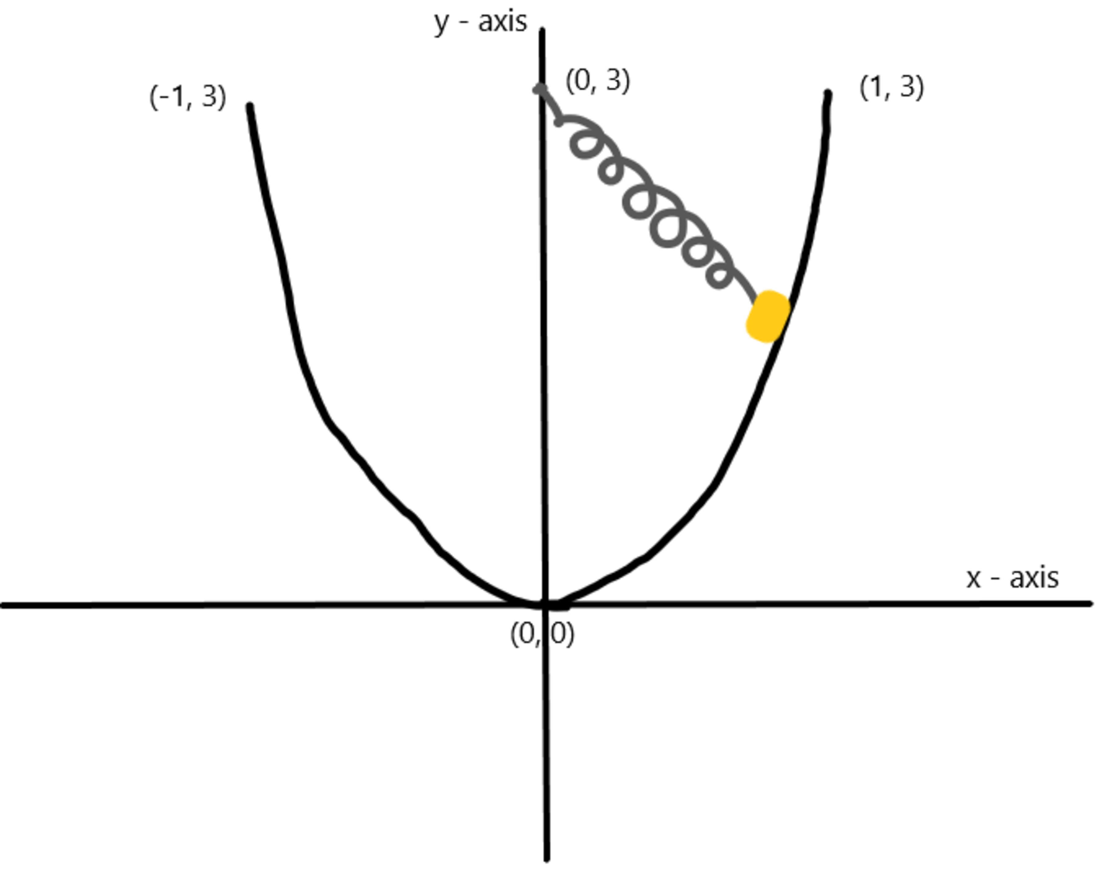
The block starts at time $t = 0$ seconds at the point $(1, 3)$ , sliding down the parabola from then on. There is friction on the parabolic ramp, and the force of the friction is $\displaystyle \mu \bold{N}$ , depending on the direction of the velocity, where $\bold{N}$ is the magnitude of the normal force to the ramp.

Here's the problem:

Find the time when the block first stops. Let that time be $t_1$ . Without stopping the timer, find the time it takes (from $t = 0$ ) for the block to stop for the second time. Let that value be $t_2$ .

Now, enter your answer as $t_1 + t_2$

Important clarifications:

The natural length of the spring is $1$ meter.
The spring constant of the spring is $10 N/m$
There is ambient gravitational acceleration, $g = 10m/s^2$ .
The mass of the block is $10 kg$
The equation of the parabola is $y = 3x^2$
The coefficient of friction of the ramp is $\mu = 0.2$

The answer is 3.67.

1 solution

Steven Chase
Jul 20, 2020

Derive an acceleration constraint equation:

$y = 3 x^2 \\ \dot{y} = 6 x \dot{x} \\ \ddot{y} = 6 x \ddot{x} + 6 \dot{x}^2$

Now write the Newton's Second Law equations. In these, $\vec{u}_1$ is the normal vector which can be calculated using standard techniques, and $\vec{u}_2$ is a unit vector in the opposite direction as the particle velocity. $\vec{F}_g$ is the gravitational force, and $\vec{F}_s$ is the spring force . $N$ is the magnitude of the normal force.

$\ddot{x} = (F_{g x} + F_{s x} + N u_{1x} + \mu N u_{2x})/m \\ \ddot{y} = (F_{g y} + F_{s y} + N u_{1y} + \mu N u_{2y})/m$

Plug these two equations into the acceleration constraint equation to solve a single equation for $N$ . Then knowing $N$ , calculate the acceleration components. This approach requires a bit of algebraic manipulation, but does not require any calls of a linear algebra routine. Numerical integration takes care of the rest.

Simulation code is attached. Results are printed at the very end.

import math

x0 = 0.0
y0 = 3.0

L0 = 1.0
k = 10.0
g = 10.0
m = 10.0
u = 0.2

dt = 10.0**(-6.0)

#####################################

x = 1.0
y = 3.0

xd = -(10.0**(-4.0))
yd = 6.0*x*xd

xdd = 0.0
ydd = 0.0

#####################################

t = 0.0
count = 0

flag = 0

while xd <= 0.0:

    x = x + xd*dt
    y = y + yd*dt

    xd = xd + xdd*dt
    yd = yd + ydd*dt

    u1x = -6.0*x
    u1y = 1.0

    u1 = math.hypot(u1x,u1y)

    u1x = u1x/u1
    u1y = u1y/u1

    v = math.hypot(xd,yd)

    u2x = -xd/v
    u2y = -yd/v

    Fgx = 0.0
    Fgy = -m*g

    Dx = x0 - x
    Dy = y0 - y

    D = math.hypot(Dx,Dy)

    dx = Dx/D
    dy = Dy/D

    s = D - L0

    Fsx = k*s*dx
    Fsy = k*s*dy

    right = -6.0*m*(xd**2.0) + Fgy + Fsy - 6.0*x*Fgx - 6.0*x*Fsx
    left = 6.0*x*u1x + 6.0*x*u*u2x - u1y - u*u2y

    N = right/left

    if N < 0.0:
        flag = 1

    xdd = (Fgx + Fsx + N*u1x + u*N*u2x)/m
    ydd = (Fgy + Fsy + N*u1y + u*N*u2y)/m

    t = t + dt
    count = count + 1

t1 = t

#####################################

print dt
print t
print ""
print x
print (y - 3.0*x*x)
print ""
print flag

print "############################"

print ""
print ""

#####################################

flag = 0

while xd >= 0.0:

    x = x + xd*dt
    y = y + yd*dt

    xd = xd + xdd*dt
    yd = yd + ydd*dt

    u1x = -6.0*x
    u1y = 1.0

    u1 = math.hypot(u1x,u1y)

    u1x = u1x/u1
    u1y = u1y/u1

    v = math.hypot(xd,yd)

    u2x = -xd/v
    u2y = -yd/v

    Fgx = 0.0
    Fgy = -m*g

    Dx = x0 - x
    Dy = y0 - y

    D = math.hypot(Dx,Dy)

    dx = Dx/D
    dy = Dy/D

    s = D - L0

    Fsx = k*s*dx
    Fsy = k*s*dy

    right = -6.0*m*(xd**2.0) + Fgy + Fsy - 6.0*x*Fgx - 6.0*x*Fsx
    left = 6.0*x*u1x + 6.0*x*u*u2x - u1y - u*u2y

    N = right/left

    if N < 0.0:
        flag = 1

    xdd = (Fgx + Fsx + N*u1x + u*N*u2x)/m
    ydd = (Fgy + Fsy + N*u1y + u*N*u2y)/m

    t = t + dt
    count = count + 1

t2 = t

#####################################

print dt
print t
print ""
print x
print (y - 3.0*x*x)
print ""
print flag

print "############################"

print ""
print ""

#####################################


print (t1+t2)


# Results

#>>> 
#1e-06
#1.36911299998

#-0.593621755566
#-2.31240470243e-05

#0
#############################


#1e-06
#2.30096599997

#0.350809601593
#-3.31317581823e-05

#0
############################


#3.67007899995
#>>>

Very brilliant solution. Can I attach the theory behind the approach I took, and is it ok if you can review it to see if it's correct? Thanks.

Krishna Karthik - 10 months, 3 weeks ago

Thanks. Sure, I can take a look. I'm going to bed fairly soon, so it may take some time. Thus far, I have assumed that you have it basically right, and that there is just some small code detail causing a problem (like the atan function, for example).

Steven Chase - 10 months, 3 weeks ago

Yes; I had originally incorrectly coded in the derivative of $3x^2$ as $2x$ . That did cause a change. Anyway, sorry to keep you. Thanks and good night.

Krishna Karthik - 10 months, 3 weeks ago

Simulating Dynamics - 4

The answer is 3.67.

1 solution

0 pending reports