Magnetic Flux (5-28-2021)
Consider the following closed curve in x y z space (coordinates are in meters).
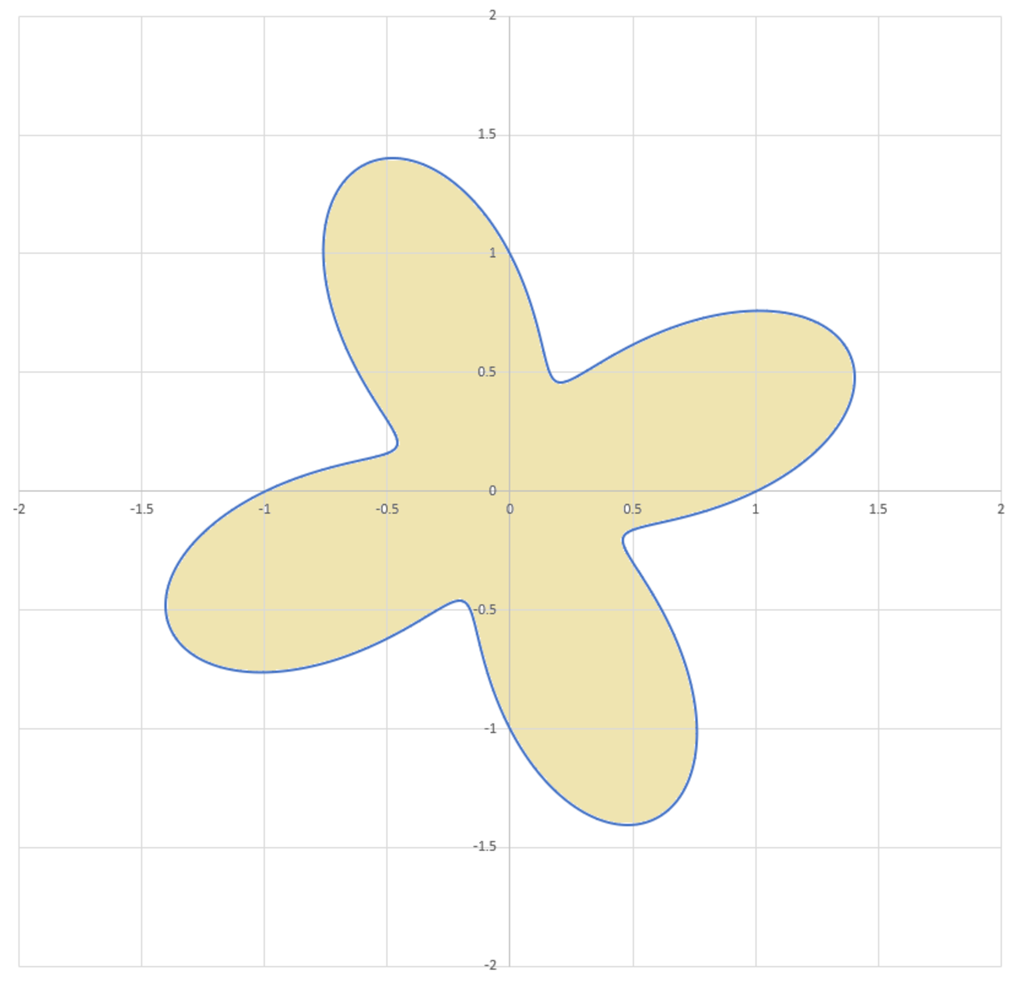
r ( θ ) x ( θ ) y ( θ ) z ( θ ) 0 ≤ = = = = θ 1 + 2 1 sin ( 4 θ ) r ( θ ) cos θ r ( θ ) sin θ θ 2 − 2 π θ ≤ 2 π
There is a magnetic flux density B throughout all of space.
B = ( B x , B y , B z ) = ( 1 , 1 , 1 ) m 2 Wb
Determine the absolute value of the magnetic flux (in Wb ) through the interior surface bounded by the curve.
∬ S B ⋅ d S
Note: The image shows the projection of the curve and interior surface onto the x y plane
The answer is 7.357.
This section requires Javascript.
You are seeing this because something didn't load right. We suggest you, (a) try
refreshing the page, (b) enabling javascript if it is disabled on your browser and,
finally, (c)
loading the
non-javascript version of this page
. We're sorry about the hassle.
1 solution
@Karan Chatrath
Hello sir.
How we will post problems now . Community will not accept more problems after 1 month
I am very worried regarding this ,share your views ?
First, the magnetic vector potential is computed using the relation:
∇ × A = B ∂ y ∂ A z − ∂ z ∂ A y = 1 ; ∂ z ∂ A x − ∂ x ∂ A z = 1 ; ∂ x ∂ A y − ∂ y ∂ A x = 1
With a little bit of trial and error, it is seen that the following vector satisfies the above relations.
A = z ( θ ) i ^ + x ( θ ) j ^ + y ( θ ) k ^
Now, by applying Stokes' theorem
Φ = ∫ ∫ S B ⋅ d S = ∫ ∫ S ( ∇ × A ) ⋅ d S = ∮ C A ⋅ d R
R = r ( θ ) cos θ i ^ + r ( θ ) sin θ j ^ + z ( θ ) k ^ d θ d R = d θ d ( r ( θ ) cos θ ) i ^ + d θ d ( r ( θ ) sin θ ) j ^ + d θ d z ( θ ) k ^ d R = ( d θ d ( r ( θ ) cos θ ) i ^ + d θ d ( r ( θ ) sin θ ) j ^ + d θ d z ( θ ) k ^ ) d θ
With the parameterisation complete, the next step is to evaluate the integrand. Here, simplifications have been left out and may be attempted by anyone interested.
Φ = ∫ 0 2 π A ⋅ d R = ∫ 0 2 π f ( θ ) d θ ⟹ ∣ Φ ∣ ≈ 7 . 3 5 6 6
The integral can be solved by outsourcing to Wolfram-Alpha or by using a script of code.