Mass Spring Equilibrium (1-6-2021)

Classical Mechanics Level 5

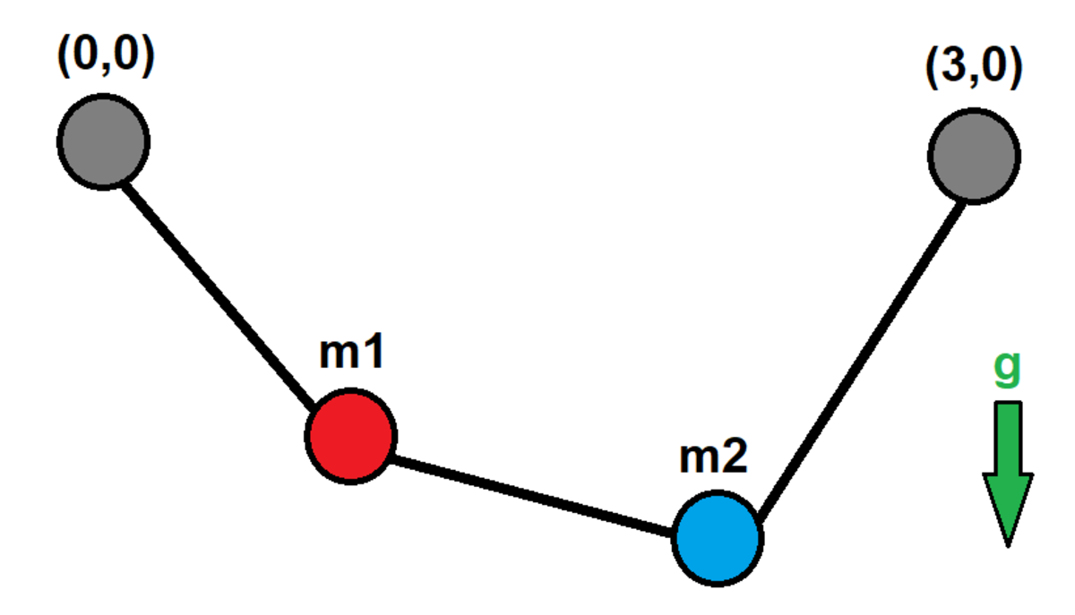
Two particles with masses $m_1$ and $m_2$ are connected by three springs as shown in the diagram. The springs are anchored at fixed points $(x,y) = (0,0)$ on the left and $(x,y) = (3,0)$ on the right. All three springs are identical, with natural length $L_0$ and force constant $k$ . The ambient gravitational acceleration $g$ is in the negative $y$ direction.

In equilibrium (zero net force on each particle), how far apart are the two particles?

Details and Assumptions:
1) $m_1 = 1$
2) $m_2 = 3$
3) $L_0 = 1$
4) $k = 5$
5) $g = 10$
6) Neglect the gravitational interaction between the particles
7) Assume appropriate standard $SI$ units for all quantities

The answer is 2.268.

4 solutions

Gediminas Sadzius
Jan 7, 2021

I'd like to share this solution where I minimised the potential energy instead of setting up a force balance. Here is a diagram explaining the variables in the potential energy function under the diagram:

$m_1\text{=}1$

$m_2\text{=}3$

$l_0\text{=}1$

$k\text{=}5$

$g\text{=}10$

The potential energy function which is to be minimised to obtain the equilibrium state of the system:

$U(\text{X1},\text{X2},\text{Y1},\text{Y2})=\frac{1}{2} k \left(\sqrt{\text{X1}^2+\text{Y1}^2}-l_0\right){}^2+\frac{1}{2} k \left(\sqrt{\text{X2}^2+(\text{Y2}-\text{Y1})^2}-l_0\right){}^2+\frac{1}{2}k\left(\sqrt{\left(\text{X3}^2+\text{Y2}^2\right.}-l_0\right){}^2+g m_1 \left(h_0-\text{Y1}\right)+g m_2 \left(h_0-\text{Y2}\right)$

In addition, the following constraint is used:

$\text{X1}+\text{X2}+\text{X3}=3$

The potential energy function is differentiated by each variable and set to zero to obtain a system of 4 equations. I took a shortcut and solved it using Wolfram Mathematica in the domain of real numbers ...

$\text{NSolve}\left[\left\{\frac{\partial U(\text{X1},\text{X2},\text{Y1},\text{Y2})}{\partial \text{X1}}=0,\frac{\partial U(\text{X1},\text{X2},\text{Y1},\text{Y2})}{\partial \text{X2}}=0,\frac{\partial U(\text{X1},\text{X2},\text{Y1},\text{Y2})}{\partial \text{Y1}}=0,\frac{\partial U(\text{X1},\text{X2},\text{Y1},\text{Y2})}{\partial \text{Y2}}\right\},\{\text{X1},\text{X2},\text{Y1},\text{Y2}\},\mathbb{R}\right]$

... to obtain just a single solution. Based on the set up of the problem its is clear the solution is the minimum:

$Y1 = 4.03487$

$Y2 = 5.93039$

$X2 = 1.24560$

The distance between the two masses is Distance = $\sqrt{\text{X2}^2+(\text{Y2}-\text{Y1})^2}$ . Plugging in the numbers gives the result $\boxed{2.268}$

@Gediminas Sadzius nice solution.upvoted.

Talulah Riley - 5 months ago

@Gediminas Sadzius Brilliant solution. I didn't think it could be solved analytically until I saw this one. Worthy of a full 3 upvotes for sure.

Krishna Karthik - 5 months ago

@Krishna Karthik thanks

Gediminas Sadzius - 5 months ago

Steven Chase
Jan 6, 2021

A few supplementary notes. There are two methods that I think are convenient for this problem.

1) Run a time-domain simulation with damping, as shown in the solution by @Karan Chatrath

2) Use a hill-climbing algorithm to randomly bump around within a four-dimensional parameter space $(x_1, y_1, x_2, y_2)$ . Store an incremental change (mutation) in the parameters if the resulting sum of the net force magnitudes $(|\vec{F}_1| + |\vec{F}_2|)$ is smaller than the smallest sum seen thus far. If not, reject the mutated parameters. Eventually the algorithm converges on the result.

I don't like Newton-Raphson for these types of problems because the symbolic manipulation is very unwieldy.

The hill-climbing algorithm code is attached

import math
import random

m1 = 1.0
m2 = 3.0

x0 = 0.0
y0 = 0.0

x3 = 3.0
y3 = 0.0

L0 = 1.0
k = 5.0

g = 10.0

########################################################################################

# Initialize mass coordinates

x1 = -10.0 + 20.0*random.random()
x2 = -10.0 + 20.0*random.random()

y1 = -10.0 + 20.0*random.random()
y2 = -10.0 + 20.0*random.random()

delta = 0.001

minres = 99999999.0

########################################################################################

for j in range(0,4*10**6):

    if j > 2*10**6:
        delta = 0.0001

    x1m = x1 + delta * (-1.0 + 2.0 * random.random())   # mutated parameters
    x2m = x2 + delta * (-1.0 + 2.0 * random.random())
    y1m = y1 + delta * (-1.0 + 2.0 * random.random())
    y2m = y2 + delta * (-1.0 + 2.0 * random.random())

    L1x = x0 - x1m                   # calculate forces
    L1y = y0 - y1m

    L2x = x2m - x1m
    L2y = y2m - y1m

    L3x = x1m - x2m
    L3y = y1m - y2m

    L4x = x3 - x2m
    L4y = y3 - y2m

    L1 = math.hypot(L1x,L1y)
    L2 = math.hypot(L2x,L2y)
    L3 = math.hypot(L3x,L3y)
    L4 = math.hypot(L4x,L4y)

    u1x = L1x/L1
    u1y = L1y/L1

    u2x = L2x/L2
    u2y = L2y/L2

    u3x = L3x/L3
    u3y = L3y/L3

    u4x = L4x/L4
    u4y = L4y/L4

    s1 = L1 - L0
    s2 = L2 - L0
    s3 = L3 - L0
    s4 = L4 - L0

    F1 = k*s1
    F2 = k*s2
    F3 = k*s3
    F4 = k*s4

    F1x = F1*u1x
    F1y = F1*u1y

    F2x = F2*u2x
    F2y = F2*u2y

    F3x = F3*u3x
    F3y = F3*u3y

    F4x = F4*u4x
    F4y = F4*u4y

    Fm1x = F1x + F2x
    Fm1y = F1y + F2y - m1*g

    Fm2x = F3x + F4x
    Fm2y = F3y + F4y - m2*g

    Fm1 = math.hypot(Fm1x,Fm1y)
    Fm2 = math.hypot(Fm2x,Fm2y)

    res = Fm1 + Fm2            # "residual" is sum of two net force magnitudes

    if res < minres:       # if mutated params give new lowest residual, keep mutation

        minres = res

        x1 = x1m 
        x2 = x2m
        y1 = y1m
        y2 = y2m 

########################################################################################

D12 = math.hypot(x1-x2,y1-y2)

if minres < 0.001:

    print minres
    print ""
    print x1
    print y1
    print ""
    print x2
    print y2
    print ""
    print D12

else:
    print "you lose, fella"

print ""
print "###########################"
print ""


#>>> 
#2.52702040261e-05

#0.918366451859
#-4.03487381439

#2.163970284
#-5.93039769329

#2.26815777276

###########################

@Steven Chase nice solution.

Talulah Riley - 5 months ago

The following code is the implementation of Newton-Raphson without crunching a single derivative by hand. Do share your thoughts or feedback. I have not commented the code properly but the general layout is hopefully understandable. I have used several user defined functions. Essentially, I am minimizing the potential energy of the system.

Run using non-zero initial coordinates. The code still has some unidentified bugs, but it seems to work otherwise.

clear all
clc

x     = [1;1;2;3];

% Newton Raphson Iteration:
for k = 1:10

     J = Jacobian(x);
     x = x - inv(J)*Potential_Gradient(x);

end

r1   = [x(1:2);0];
r2   = [x(3:4);0];
ANSWER   = norm(r2 - r1)
% ANSWER = 2.2682


%%%%%%%%%%%%%%%%%%%%%%%%%%%%%%%%%%%%%%%%%%%%%%%%%%%%%%%%%%%%%%%%%%%%%%%%%%%
% Function to calculate potential energy:

function V = Potential_Energy(X)

x1 = X(1);
y1 = X(2);
x2 = X(3);
y2 = X(4);

m1     = 1;
m2     = 3;
K      = 5;
g      = 10;
Lo     = 1;

V      = m1*g*y1 + m2*g*y2 + 0.5*K*(sqrt(x1^2+y1^2)-Lo)^2 + ...
    0.5*K*(sqrt((x2 - x1)^2+(y2 - y1)^2)-Lo)^2 + 0.5*K*(sqrt((3 - x2)^2+y2^2)-Lo)^2;
end

%%%%%%%%%%%%%%%%%%%%%%%%%%%%%%%%%%%%%%%%%%%%%%%%%%%%%%%%%%%%%%%%%%%%%%%%%%%
% Function to calculate potential energy gradient:

function F = Potential_Gradient(X)

    eps   = 1e-9;
    epsM  = eps*eye(length(X));

    for k = 1:length(X)

        X_d      = X + epsM(:,k);

        J(:,k)   = (Potential_Energy(X_d) - Potential_Energy(X))/eps;
    end

    F   = J';
end

%%%%%%%%%%%%%%%%%%%%%%%%%%%%%%%%%%%%%%%%%%%%%%%%%%%%%%%%%%%%%%%%%%%%%%%%%%%
% Function to calculate jacobian matrix of the potential gradient:

function J = Jacobian(x)

    eps   = 1e-3;
    epsM  = eps*eye(length(x));

    for k = 1:length(x)

        x_d      = x + epsM(:,k);

        J(:,k)   = (Potential_Gradient(x_d) - Potential_Gradient(x))/eps;
    end

end

Karan Chatrath - 5 months ago

So lines 40-58 are effectively setting up a system of equations by partially differentiating the potential function with respect to the four spatial parameters. And lines 58 and onward are forming the Jacobian matrix by partially differentiating each of the four equations by each of the spatial parameters. But it's all done numerically instead of analytically.

Is that a correct interpretation? If so, it's eye-opening that it can be done numerically in such a general fashion.

Steven Chase - 5 months ago

Yes, that is the correct interpretation. Symbolic manipulations can be explicitly avoided, through robust numerical techniques. However, my code is not very robust, to be honest. Work in progress.

Karan Chatrath - 5 months ago

@Steven Chase Hey, nice solution. Good problem.

Krishna Karthik - 5 months ago

Karan Chatrath
Jan 6, 2021

Equilibrium problems can generally be solved by balancing all forces or by minimizing the total potential energy of the system. I chose a dynamic route. I decided to simulate the motion in the presence of one dissipative force, from an arbitrary initial condition. The particle, after a long time, settles at its stable equilibrium position.

Let the coordinates of $m1$ be $\vec{r}_1=(x_1,y_1)$ and that of $m2$ be $\vec{r}_1=(x_2,y_2)$ . I define a drag coefficient $C_d=50$ for each mass. The drag force on each mass is:

$\vec{F}_{D1} = -C_d \lvert \vec{v}_1 \rvert \vec{v}_1$ $\vec{F}_{D2} = -C_d \lvert \vec{v}_2 \rvert \vec{v}_2$ $\vec{v}_1 = \frac{d \vec{r}_1}{dt}$ $\vec{v}_2 = \frac{d \vec{r}_2}{dt}$

Gravitational force acting on the particle:

$\vec{F}_{G1} = -m_1g \ \hat{j}$ $\vec{F}_{G2} = -m_2g \ \hat{j}$

Spring force for spring joining $m_1$ and origin:

$\vec{F}_{S1} = \left(\frac{K\left( \lvert \vec{r}_1 \rvert - L_o\right)}{\lvert \vec{r}_1 \rvert}\right)\vec{r}_1$

Spring force for spring joining $m_1$ and $m_2$ :

$\vec{F}_{S2} = \left(\frac{K\left( \lvert \vec{r}_2 - \vec{r}_1 \rvert - L_o\right)}{\lvert \vec{r}_2 - \vec{r}_1\rvert}\right)(\vec{r}_2 - \vec{r}_1)$

Spring force for spring joining $\vec{r}_f=(3,0)$ and $m_2$ :

$\vec{F}_{S3} = \left(\frac{K\left( \lvert \vec{r}_2 - \vec{r}_f \rvert - L_o\right)}{\lvert \vec{r}_2 - \vec{r}_f\rvert}\right)(\vec{r}_2 - \vec{r}_f)$

Finally, the equations of motion of the system are:

$m_1 \left[\begin{matrix} \ddot{x}_1\\ \ddot{y}_1\end{matrix} \right] =\vec{F}_{G1} + \vec{F}_{D1} -\vec{F}_{S1}+ \vec{F}_{S2}$ $m_2 \left[\begin{matrix} \ddot{x}_2\\ \ddot{y}_2\end{matrix} \right] =\vec{F}_{G2} + \vec{F}_{D2} -\vec{F}_{S2}- \vec{F}_{S3}$

Writing out the equations of motion requires a rough free body diagram, which I have left out. The reader may attempt to derive these and see if they agree with my findings. Finally, this system can be numerically integrated for a prolonged period of time till the drag force dissipates all energy out of the system, leaving it in its state of minimal potential energy. In fact, equating the the accelerations to zero and assuming the system to be in rest gives the equilibrium equations itself. That requires an iterative scheme like Newton-Raphson to solve.

Simulation code attached below:

clear all, clc

% Parameters:
m1     = 1;
m2     = 3;
g      = 10;
Lo     = 1;
K      = 5;
Cd     = 50;

% Time initialisation:
dt     = 1e-4;
tf     = 200;
t      = 0:dt:tf;

% initial conditions:
x1(1)  = 1;
y1(1)  = 0;
x2(1)  = 2;
y2(1)  = 0;

dx1(1) = 0;
dy1(1) = 0;
dx2(1) = 0;
dy2(1) = 0;


for k = 1:length(t)-1

    % Length of springs:
    Ls1     = sqrt((x1(k)-0)^2 + (y1(k)-0)^2);
    Ls2     = sqrt((x2(k)-x1(k))^2 + (y2(k)-y1(k))^2);
    Ls3     = sqrt((x2(k)-3)^2 + (y2(k)-0)^2);

    % Spring elongations:
    Le1     = Ls1 - Lo;
    Le2     = Ls2 - Lo;
    Le3     = Ls3 - Lo;

    % Drag forces:
    Fd1     = -Cd*norm([dx1(k);dy1(k);0])*[dx1(k);dy1(k)];
    Fd2     = -Cd*norm([dx2(k);dy2(k);0])*[dx2(k);dy2(k)];

    % Gravity:
    Fg1     = [0;-m1*g];
    Fg2     = [0;-m2*g];

    % Spring forces (visualise directions):
    Fs1     = (K*Le1*[x1(k);y1(k)])/Ls1;
    Fs2     = (K*Le2*[x2(k)-x1(k);y2(k)-y1(k)])/Ls2;
    Fs3     = (K*Le3*[x2(k)-3;y2(k)-0])/Ls3;

    % Equations of motion:
    ddr1    = (Fg1 + Fd1 - Fs1 + Fs2)/m1;
    ddr2    = (Fg2 + Fd2 - Fs2 - Fs3)/m2;

    % Numerical integration - Semi implicit Euler:
    dx1(k+1) = dx1(k) + ddr1(1)*dt;
    dy1(k+1) = dy1(k) + ddr1(2)*dt;

    dx2(k+1) = dx2(k) + ddr2(1)*dt;
    dy2(k+1) = dy2(k) + ddr2(2)*dt;

    x1(k+1)  = x1(k) + dx1(k+1)*dt;
    y1(k+1)  = y1(k) + dy1(k+1)*dt;

    x2(k+1)  = x2(k) + dx2(k+1)*dt;
    y2(k+1)  = y2(k) + dy2(k+1)*dt;
end

r1_end = [x1(end);y1(end);0];
r2_end = [x2(end);y2(end);0];

ANSWER = norm(r2_end - r1_end)
% ANSWER = 2.2683

Hehe, good one. I solved it exactly the same way. At first I tried screwing around with simultaneous equations, but realised that the equations were too complicated to solve.

Krishna Karthik - 5 months ago

Krishna Karthik
Jan 10, 2021

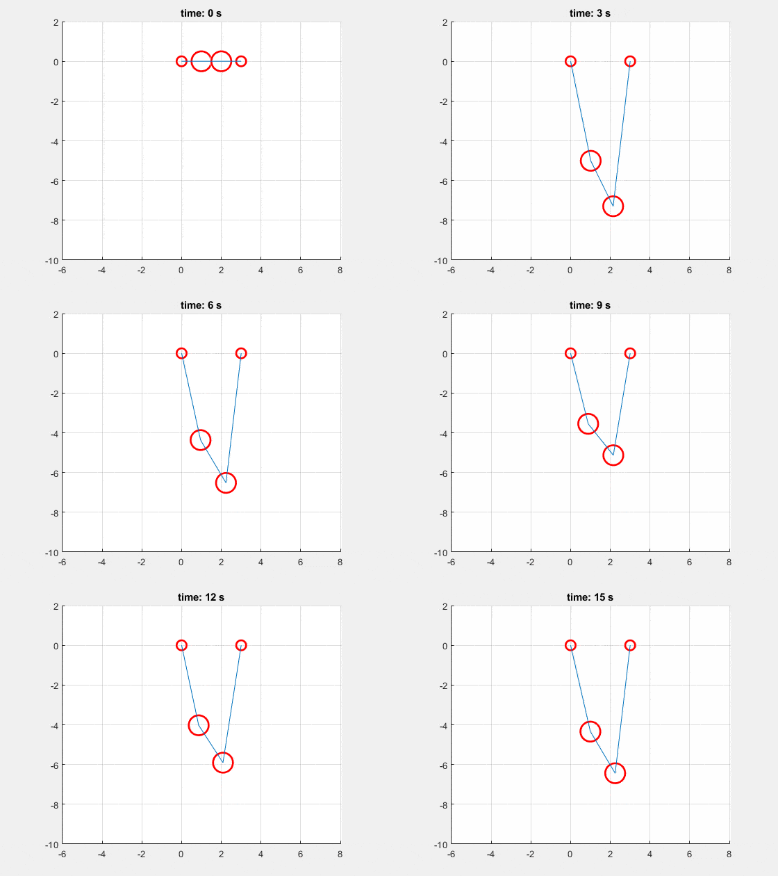
My code is almost exactly the same as Karan Chatrath's, so I don't have much to add. I approached the problem the same way by adding damping and computing all the force vectors and numerically integrating.

Although I attempted the problem analytically at first by making a system of 4 equations, the equations were way too complicated to solve.

So I simulated the motion over a long period of time.

Here are some juicy gifs:

Mass Spring Equilibrium (1-6-2021)

The answer is 2.268.

4 solutions

0 pending reports