Measurement of a radioactive decay

A specimen is activated by the bombardment with neutrons, so that the sample itself becomes radioactive for a short time and releases beta radiation. The radioactivity of the activated specimen is then measured with a Geiger counter. The Geiger counter is located at a distance of from the radiating specimen and detects all particles that hit its circular front surface with the diameter . The radioactive sample is point-shaped and radiates homogeneously in all spatial directions.
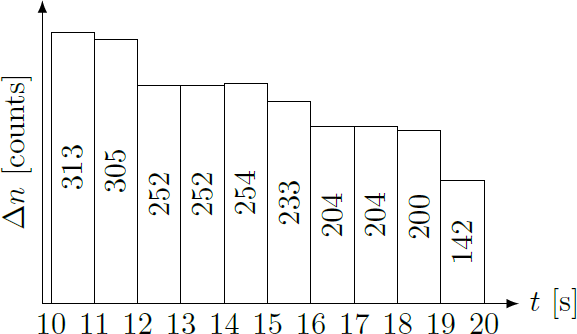
Each beta particle detected by the Geiger counter is electronically counted. The decays are summed up in the time interval of one second each. In the time range between 10 and 20 seconds after activation, the following statistics result:
What is the approximate number of radioactive atoms in the sample at the time ?
Assumptions: The number of the radioactive atoms follows the decay law with the initial number and the decay constant . The scattering and absorption of beta particles in the air is negligible. Other radiation sources are negligible. The Geiger counter has an efficiency of 100%, so that all incoming beta particles are counted.
This section requires Javascript.
You are seeing this because something didn't load right. We suggest you, (a) try
refreshing the page, (b) enabling javascript if it is disabled on your browser and,
finally, (c)
loading the
non-javascript version of this page
. We're sorry about the hassle.
The number A of beta particles per second (activity) correspond to the decay rate of the radioactive atoms A = − N ˙ = λ N 0 exp ( − λ t ) The radiation is homogeneously distributed over the whole sphere with area S 0 = 4 π r 2 . The Geiger counter detects only the particles inside the area S = π d 2 / 4 , so that the mean counting rate is n ˙ = S 0 S A = 1 6 r 2 d 2 λ N 0 exp ( − λ t ) The total number of counts, Δ n , for a time intervall Δ t = 1 s can be approximated by Δ n ≈ n ˙ Δ t provided that Δ t ≪ 1 / λ applies. For the logarithmic number lo g ( Δ n ) results in a linear time dependence lo g ( Δ n ) ⇒ N 0 = lo g ( 1 6 r 2 d 2 λ N 0 Δ t ) − λ t = A + B ⋅ t = − d 2 Δ t 1 6 r 2 B exp ( A ) So, if you present the results as a semi-logarithmic plot, you can use points to draw a regression line:
In this case, the regression line correspond to the parameters A B ⇒ N 0 ≈ 6 . 5 2 ± 0 . 1 4 ≈ − 0 . 0 7 1 8 ± 0 . 0 0 9 3 s 1 ≈ ( 0 . 9 ± 0 . 2 ) ⋅ 1 0 9