Method of image charges (part II)
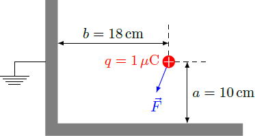
An electrical charge q = 1 μ C is located near two grounded metal plates that are welded together in an right angle. The distances between the charge and the metal surfaces are a = 1 0 cm and b = 1 8 cm .
What is the magnitude of the electrostatic force F = ∣ F ∣ , that is exerted by the metal plates on the charge q ?
Give the result in units of Newton. The vacuum permittivity is ε 0 ≈ 8 . 8 5 4 ⋅ 1 0 − 1 2 F / m .
Hint: Look for a configuration of image charges, so that both metal surfaces are equipotential surfaces.
This problem is part of a series on the method of image charges. The first part can be reached via this link .
The answer is 0.2.
This section requires Javascript.
You are seeing this because something didn't load right. We suggest you, (a) try
refreshing the page, (b) enabling javascript if it is disabled on your browser and,
finally, (c)
loading the
non-javascript version of this page
. We're sorry about the hassle.
2 solutions
By the method of the image charges, the following image charge arrangement can be made
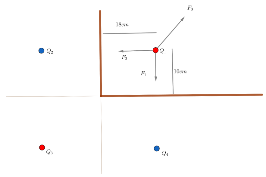
In the picture above the red dots represent positive charge and the blue dots represent the negative and all charges have equal magnitude of q = 1 μ C
Now from the Coulomb's law we have(as shown in the above picture):
F 1 = 4 π ϵ 0 ( 2 a ) 2 − q 2 a y
F 2 = 4 π ϵ 0 ( 2 b ) 2 − q 2 a x
F 2 = 4 π ϵ 0 ( ( 2 a ) 2 + ( 2 b ) 2 ) 2 3 − q 2 ( a x 2 b + a y 2 a )
So now we have F = F 1 + F 2 + F 3
⇒ F = 1 6 π ϵ 0 q 2 [ a x ( ( a 2 + b 2 ) 2 3 b − b 2 1 ) + a y ( ( a 2 + b 2 ) 2 3 a − a 2 1 ) ]
⇒ ∣ F ∣ = 1 6 π ϵ 0 q 2 [ ( ( a 2 + b 2 ) 2 3 b − b 2 1 ) ] 2 + [ ( ( a 2 + b 2 ) 2 3 a − a 2 1 ) ] 2
Now putting the known values:
a = 1 0 cm
b = 1 8 cm
q = 1 μ C
ε 0 ≈ 8 . 8 5 4 ⋅ 1 0 − 1 2 F / m ,
We get F = 0 . 2 0 0 2 8 5 4 0 1 4 3 ≈ 0 . 2
The charge and three image charges are symmetrical arranged around the origin in an rectangle with alternating signs. The charges can be grouped into two dipoles with a common perpendicular bisector at x = 0 or y = 0 such that ϕ ( 0 , y ) = ϕ ( x , 0 ) = 0 and the metal surface is an equipotential surface as required.
All four charges together create a potential ϕ ( x , y ) = 4 π ε 0 1 i = 0 ∑ 3 ∣ r − r i ∣ q i = 4 π ε 0 q n = ± 1 ∑ m = ± 1 ∑ ( x − n a ) 2 + ( y − m b ) 2 n m where r 0 = ( a , b ) is the position vector of the actual charge. You can easily calculate that ϕ ( 0 , y ) = ϕ ( x , 0 ) = 0 .
The electric field E ( x , y ) of the image charges results E ( x , y ) = 4 π ε 0 q ⎣ ⎢ ⎢ ⎡ [ ( x + a ) 2 + ( y + b ) 2 ] 3 / 2 ( x + a y + b ) − [ ( x − a ) 2 + ( y + b ) 2 ] 3 / 2 ( x − a y + b ) − [ ( x + a ) 2 + ( y − b ) 2 ] 3 / 2 ( x + a y − b ) ⎦ ⎥ ⎥ ⎤ Thus, the charge q at r = ( x , y ) = ( a , b ) experiences a force F = q E ( a , b ) = 4 π ε 0 q 2 [ 8 [ a 2 + b 2 ] 3 / 2 1 ( 2 a 2 b ) − 8 b 3 1 ( 0 2 b ) − 8 a 3 1 ( 2 a 0 ) ] = − 1 6 π ε 0 q 2 ( 1 / a 2 − a / [ a 2 + b 2 ] 3 / 2 1 / b 2 − b / [ a 2 + b 2 ] 3 / 2 ) If we plug in the numbers, we get the final result F ∣ F ∣ ≈ ( − 0 . 1 9 9 − 0 . 0 2 3 ) N = F x 2 + F y 2 ≈ 0 . 2 N