Noisy regression
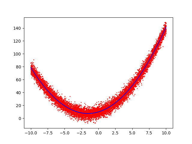
Real-world data is noisy. When performing an experiment, this data was measured.
If we are expecting the result to be a parabola of the form y = a ⋅ x 2 + b ⋅ x + c , find a , b , and c that minimize the mean-squared error.
Enter the answer as a + b + c .
Note: There are tools that make this job automagically like origin, but we are here for the learning purpose and it would be a good exercise to implement this at least once to understand how those tools work.
The answer is 14.021535716869955.
This section requires Javascript.
You are seeing this because something didn't load right. We suggest you, (a) try
refreshing the page, (b) enabling javascript if it is disabled on your browser and,
finally, (c)
loading the
non-javascript version of this page
. We're sorry about the hassle.
2 solutions
Hello sir, very nice solution, though in the last equation, shouldnt the letter above the sigma be n instead of m?
It is well known that if we have 3 points we can define a parabola with the following matrix
⎣ ⎡ y 0 y 1 y 2 ⎦ ⎤ = ⎣ ⎡ x 0 2 x 1 2 x 2 2 x 0 x 1 x 2 1 1 1 ⎦ ⎤ ⋅ ⎣ ⎡ a b c ⎦ ⎤
or more commonly written as A x = b where
A = ⎣ ⎡ x 0 2 x 1 2 x 2 2 x 0 x 1 x 2 1 1 1 ⎦ ⎤ , x = ⎣ ⎡ a b c ⎦ ⎤ , b = ⎣ ⎡ y 0 y 1 y 2 ⎦ ⎤
and we can calculate x by computing x = A − 1 b .
Well, we do have three points but we have even more than 3 points but, because the data is noisy, is not likely that any 2 triplets will fit to the same parabola, and if we are to include all points, our matrix A is not square, so we can't invert it. It turns out that there is a notion of a pseudo-inverse that can be applied to m × n matrix and when applied it has the nice property of minimizing the squared error and it is defined by ( A T A ) − 1 A T so we can compute x by computing x = ( A T A ) − 1 A T b . Here is my python implementation of it with the plot of the data and the regression line:
1 2 3 4 5 6 7 8 9 10 11 12 13 14 15 16 17 18 19 |
|

It is worth noting that, with your matrices A = ⎝ ⎜ ⎜ ⎛ x 1 2 x 2 2 ⋯ x n 2 x 1 x 2 ⋯ x n 1 1 ⋯ 1 ⎠ ⎟ ⎟ ⎞ b = ⎝ ⎜ ⎜ ⎛ y 1 y 2 ⋯ y n ⎠ ⎟ ⎟ ⎞ then n A T A = ⎝ ⎛ E [ x 4 ] E [ x 3 ] E [ x 2 ] E [ x 3 ] E [ x 2 ] E [ x ] E [ x 2 ] E [ x ] 1 ⎠ ⎞ n A T b = ⎝ ⎛ E [ x 2 y ] E [ x y ] E [ y ] ⎠ ⎞ and so your method is in fact the same as mine. This explains why your method works.
Log in to reply
Pretty much, I loved your approach to it but yeah, they are in fact equivalent.
If we want to minimize F ( a , b , c ) = j = 1 ∑ n ( y j − a x j 2 − b x j − c ) 2 then we require ∂ a ∂ F = ∂ b ∂ F = ∂ c ∂ F = 0 and hence ⎝ ⎛ E [ x 4 ] E [ x 3 ] E [ x 2 ] E [ x 3 ] E [ x 2 ] E [ x ] E [ x 2 ] E [ x ] 1 ⎠ ⎞ ⎝ ⎛ a b c ⎠ ⎞ = ⎝ ⎛ E [ x 2 y ] E [ x y ] E [ y ] ⎠ ⎞ where E [ x m ] = n 1 j = 1 ∑ n x j m 1 ≤ m ≤ 4 is the average value of x m for the data, and E [ x m y ] = n 1 j = 1 ∑ m x j m y j 0 ≤ m ≤ 2 is the average value of x m y for the data (note that n is the number of data points - in this case, n = 1 0 0 0 0 ).
Calculating these expected values can be done easily in Excel, and simple Gaussian elimination solves the equation, giving a = 1 . 0 0 3 0 8 9 3 2 2 , b = 3 . 1 3 2 9 6 1 8 5 5 , c = 9 . 8 8 5 4 8 4 5 4 , obtaining a + b + c = 1 4 . 0 2 1 5 3 5 7 2 .