Nonlinear Resonance - Guided Exercise

Classical Mechanics Level 5

A spring-mass-damper system is equipped with a nonlinear spring. The potential energy as a function of deformation $x$ of the spring relative to its natural length is:

$V(x) = \frac{\omega^2 x^2}{2} +\frac{\delta x^4}{4}$

The magnitude of damping force is given by the following and it acts opposite to the direction of motion of the mass.

$F_D = \lvert D\dot{x} \rvert$

At time $t=0$ , the mass is at rest and the spring is un-deformed ( $x=0$ ). An external force $F_{\mathrm{ext}}=\sin(\omega_{\mathrm{ext}} t)$ starts to act on the system at $t=0$ along the axis of the spring. Find the resonant frequency ( $\omega_{\mathrm{ext}}$ ) of this system. Enter your answer in $\mathrm{rad/s}$ .

Guidelines to solve:

The frequency of the external force was varied in steps of $0.01 \ \mathrm{rad/s}$ when I solved it numerically.
All time domain simulations (if necessary) were run for 100 seconds with a time step of $10^{-3}$ .
$\omega^2 = 2$ , $m = 1$ , $D = 0.05$ , $\delta = 0.01$
All quantities are in SI units.
Neglect gravity.
Caution - The reason why I mention the solution specifics is because this problem can otherwise become computationally very expensive. The solver is recommended to stick to the aforementioned numerical guidelines. This problem can also be attempted using perturbation techniques as the nonlinearity is weak.

Bonus: Compare the resonant frequency of the linear case ( $\delta=0$ ) with this weakly nonlinear system. Demonstrate the effect of nonlinearity in a plot. Compare your result with other values of $\delta$ .

The answer is 1.54.

2 solutions

Mark Hennings
Dec 22, 2020

Using Mathematica, we define

MyY[t_] := ParametricNDSolveValue[{y''[t] + 0.05y'[t] + 2y[t] + 0.01y[t]^3 == Sin[w t],y[0] == 0,y'[0] == 0},y,{t,0,100},{w}}

MaxMyY[w_] := NMaximize[{Abs[MyY[w][t]],0 <= t <= 100},t][[1]]

Plotting $\mathrm{MaxMyY}$ against $w$ gives the graph

It is interesting that (ignoring small numerical errors) the value of $\mathrm{MaxMyY}$ builds up steadily to its peak value, and then collapses abruptly. I make the critical resonant angular frequency equal to $\boxed{1.54002}$ to $5$ DP.

Thanks for the solution and especially for the animated plot. I also observed the abrupt jump in the frequency response. However, my understanding of this effect of nonlinearity is limited at the moment.

Karan Chatrath - 5 months, 3 weeks ago

Steven Chase
Dec 21, 2020

The spring force is:

$F_s (x) = - \frac{d}{dx} V(x) = -(\omega^2 x + \delta x^3)$

The simulation outline is as follows:

1) Sweep $\omega_{ext}$ from $0$ to $10$ in increments of $0.01$ .

2) For each $\omega_{ext}$ , run a time domain simulation from $t = 0$ to $t = 100$ . For the $\delta = 0.01$ case, I used a time step of $10^{-4}$ , and for other values of $\delta$ , I used a time step of $10^{-3}$ . With a $10^{-4}$ time step, the simulation time is quite large.

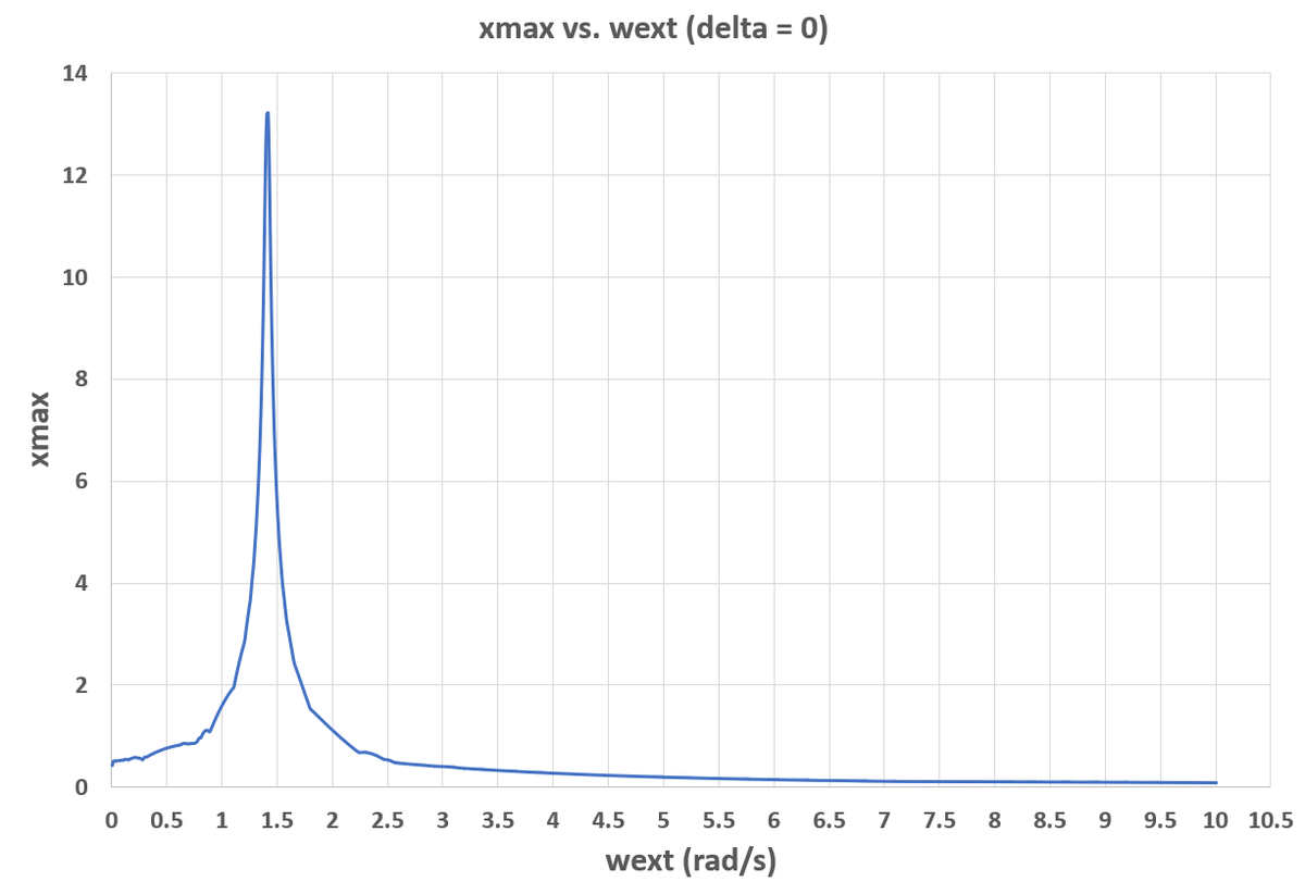
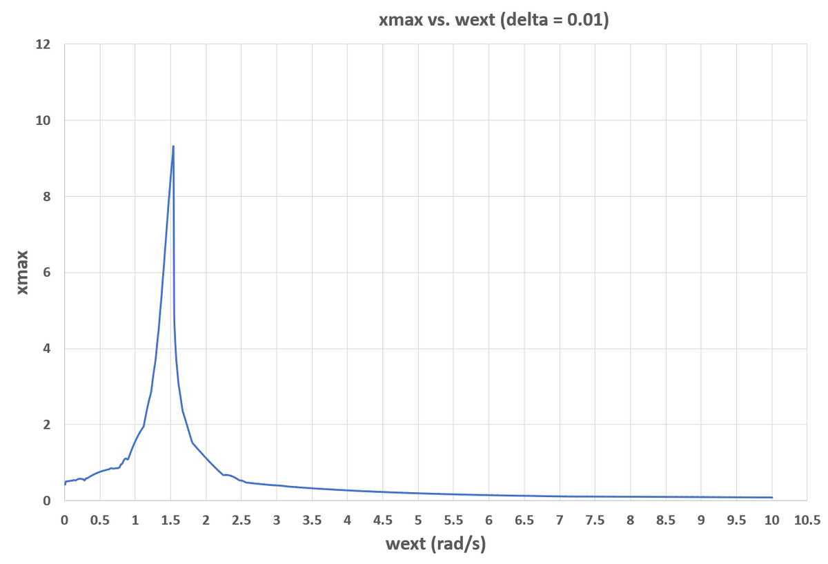
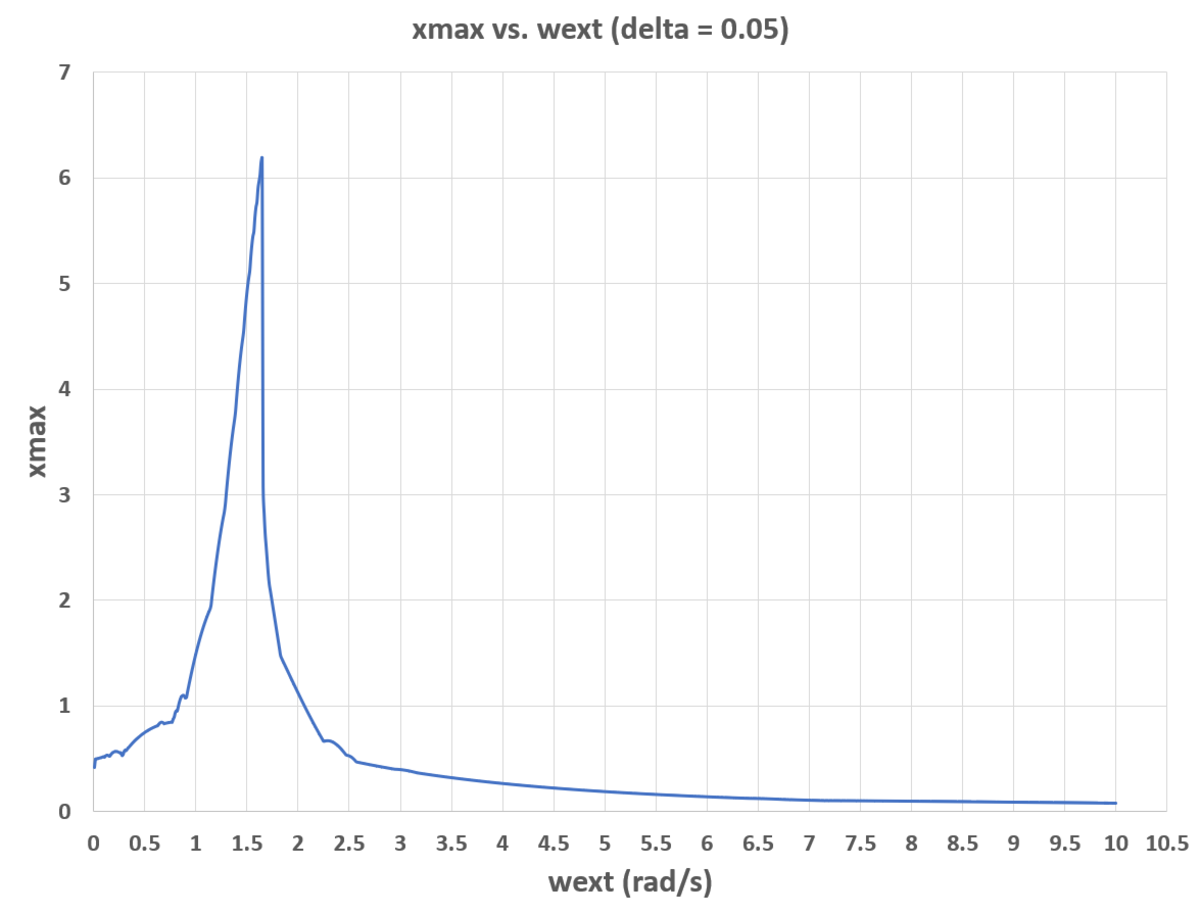
3) For each $\omega_{ext}$ , keep track of the largest value of $x$ ( $x_{max})$ which occurs during the time domain simulation. The resonant frequency is the value of $\omega_{ext}$ that has the largest $x_{max}$ .

It appears that larger $\delta$ results in a larger resonant frequency. For $\delta = 0$ , the resonant frequency is $1.42$ . For $\delta = 0.01$ , the resonant frequency is $1.54$ . For $\delta = 0.05$ , the resonant frequency is $1.65$ . Plots and simulation code are below.

Plots:

Simulation Code:

import math

dt = 10.0**(-3.0)
dwext = 0.01
tf = 100.0

wsq = 2.0
m = 1.0
D = 0.05
delta = 0.05

###################################

wext = dwext

while wext <= 10.0:

    t = 0.0
    x = 0.0
    xd = 0.0
    xdd = 0.0

    xmax = 0.0

    while t <= tf:

        x = x + xd*dt
        xd = xd + xdd*dt

        Fs = -(wsq*x + delta*(x**3.0))

        Fext = math.sin(wext*t)

        FD = -D*xd

        F = Fs + FD + Fext

        xdd = F/m

        if x > xmax:
            xmax = x

        t = t + dt

    print wext,xmax


    wext = wext + dwext

Thanks for the solution. If you plot the frequency responses for each $\delta$ one atop another, it will be observed that introduction of the nonlinearity tilts the response one way or another depending on the sign of $\delta$ . This observation is just as a result of a weak nonlinearity, which I find remarkable. Real systems exhibit stronger nonlinearities and hence more skewed frequency responses. I am still trying to develop a physical intuition of nonlinear vibrations. Linearity in nature is truly an aberration.

Moreover, the linear case agrees with our expectation of the resonant frequency being $\sqrt{2}$ .

An analogous electrical circuit would be a series RLC with a nonlinear capacitor. I wonder what the physical implications would be there.

Karan Chatrath - 5 months, 3 weeks ago

Is the formula in this problem representative of a real-world spring, as far as the form of the equation goes?

Steven Chase - 5 months, 3 weeks ago

Think of a damped driven pendulum. The equation of motion is:

$\ddot{\theta} + D\dot{\theta} + \frac{g}{L}\sin{\theta}=T_{\mathrm{ext}}$

Now, we usually make a small angle approximation where $\sin{\theta} \approx \theta$ . Taking higher degree terms of the sine series, one can also represent the equation of motion as:

$\ddot{\theta} + D\dot{\theta} + \frac{g}{L}\left(\theta - \frac{\theta^3}{3!}\right)=T_{\mathrm{ext}}$

I do not know of a specific spring model having cubic nonlinearity, but I can say with some certainty that the Hooke's law model of a spring is in many occasions, inadequate to model reality.

Karan Chatrath - 5 months, 3 weeks ago

Nonlinear Resonance - Guided Exercise

The answer is 1.54.

2 solutions

0 pending reports