Numerical Stability of Euler Variants
Consider the classic explicit Euler numerical integration technique:
x k = x k − 1 + x ˙ k − 1 Δ t
And a modified version:
x k = x k − 1 + x ˙ k − 1 Δ t + x ¨ k − 1 ( Δ t ) 2
Suppose we use these to discretely approximate the following continuous-time signal:
x ( t ) = e α t
In the above equation, α is a complex number. Define "stability" as the following being true for all processing steps:
∣ ∣ ∣ x k − 1 x k ∣ ∣ ∣ < 1
For each integration method, determine the region of stability in the complex α plane, as well as the area of each region.
For Δ t = 1 , what is the following ratio?:
Area of explicit Euler stability region Area of modified Euler stability region
Bonus: Make scatter plots of both stability regions. Actually, this is the best way to map out the stability regions anyway
The answer is 0.8394.
This section requires Javascript.
You are seeing this because something didn't load right. We suggest you, (a) try
refreshing the page, (b) enabling javascript if it is disabled on your browser and,
finally, (c)
loading the
non-javascript version of this page
. We're sorry about the hassle.
1 solution
Indeed, by "stable" I just mean "doesn't blow up". As you say, there are some exponentially increasing signals that will exponentially decrease when numerically approximated. So the results for those cases are bogus. Similarly, there are exponentially decaying signals that will exponentially grow when numerically approximated. The trapezoidal method, by contrast, contains the entire left plane and nothing in the right plane.
Log in to reply
True. The bottom line is that all numerical techniques are (eventually) inaccurate, and that errors accumulate. The question is how fast the methods diverge from the actual value, enabling a cost-benefit analysis conversation about how small h = Δ t must be to enable an acceptable level of error, given that a smaller value of h will require more iterations. The trapezoidal technique has a cubic local truncation error, so the rate of divergence from the actual value is proportional to h 3 instead of h ; this makes it better than other schemes, but still inaccurate if pushed too far.
Since x ˙ = α x and x ¨ = α 2 x , the explicit Euler formula in this case is simply x k = ( 1 + α ) x k − 1 and hence the stability condition is ∣ 1 + α ∣ < 1 . Thus α lies in the disk with centre − 1 and radius 1 , and hence the explicit stability region has area π .
On the other hand, the modified formula is simply x k = ( 1 + α + α 2 ) x k − 1 which means that the stability condition is ∣ ∣ ∣ ( α + 2 1 ) 2 + 4 3 ∣ ∣ ∣ = ∣ α 2 + α + 1 ∣ < 1 which means that ( α + 2 1 ) 2 must lie in the circle with centre − 4 3 and radius 1 . In polar coordinates this means that ( α + 2 1 ) 2 = r e i θ where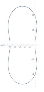 0
≤
r
<
4
1
(
7
+
9
cos
2
θ
−
3
cos
θ
)
−
π
≤
θ
≤
π
Thus we deduce that
α
=
r
e
i
θ
−
2
1
where
0
≤
r
<
R
(
θ
)
=
2
1
7
+
9
cos
2
2
θ
−
3
cos
2
θ
−
π
≤
θ
≤
π
A graph of the modified stability region is shown. Its area is
4
∫
0
2
1
π
2
1
R
(
θ
)
2
d
θ
=
2
1
∫
0
2
1
π
(
7
+
9
cos
2
2
θ
−
3
cos
2
θ
)
d
θ
=
2
E
(
1
6
9
)
where
E
is the complete elliptic integral. This makes the ratio of areas
π
2
E
(
1
6
9
)
=
0
.
8
3
9
3
6
5
. No scatter diagrams required.
0
≤
r
<
4
1
(
7
+
9
cos
2
θ
−
3
cos
θ
)
−
π
≤
θ
≤
π
Thus we deduce that
α
=
r
e
i
θ
−
2
1
where
0
≤
r
<
R
(
θ
)
=
2
1
7
+
9
cos
2
2
θ
−
3
cos
2
θ
−
π
≤
θ
≤
π
A graph of the modified stability region is shown. Its area is
4
∫
0
2
1
π
2
1
R
(
θ
)
2
d
θ
=
2
1
∫
0
2
1
π
(
7
+
9
cos
2
2
θ
−
3
cos
2
θ
)
d
θ
=
2
E
(
1
6
9
)
where
E
is the complete elliptic integral. This makes the ratio of areas
π
2
E
(
1
6
9
)
=
0
.
8
3
9
3
6
5
. No scatter diagrams required.
Is the term "stability" suitable in this second case? As can be seen, the "stability region" contains numbers with positive real part, and hence for which ∣ x ( k ) ∣ will diverge to ∞ as k → ∞ . Since we are trying to approximate x ( k ) by x k , we don't want ∣ x k + 1 ∣ < ∣ x k ∣ in this case, do we?