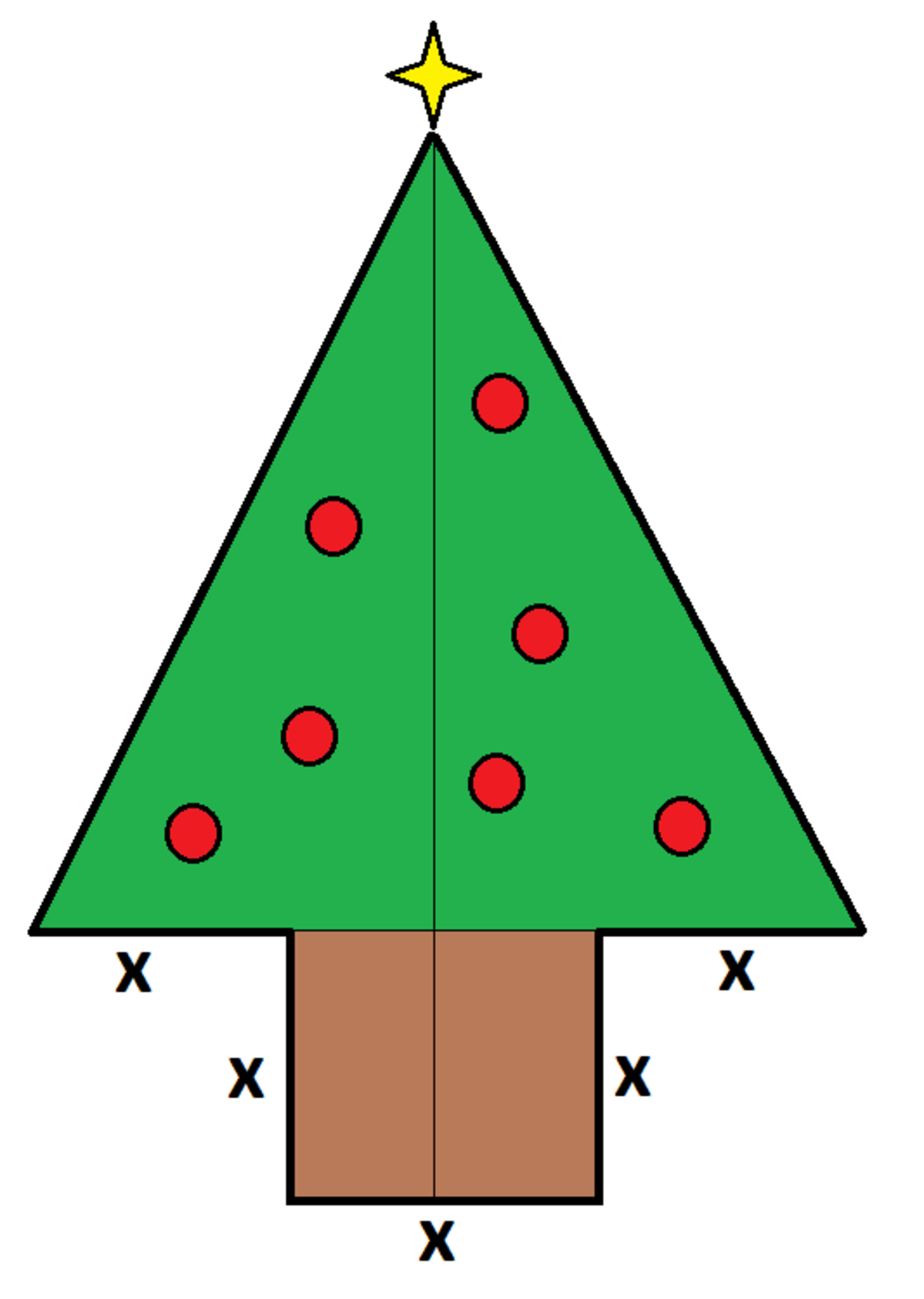
O Tannenbaum, How Optimal Thine Area

Greetings and best wishes to you these holidays!

Let the height of the green isosceles triangle be $h$ . Then the perimeter is:

$P = 5x + 2\sqrt{\left(x+\frac{x}{2}\right)^2 + h^2} \implies P = 5x + \sqrt{9x^2 + 4h^2}$

The area of the triangle is:

$A = x^2 + \frac{3}{2}xh$

Method 1: Given that the perimeter is the constraint, the cost function, with the introduction of a Lagrange multiplier can be formulated as such:

$L = A + \lambda (P-100)$

To be more rigorous, two more Lagrange multipliers are to be introduced to account for the inequality constraints $(0 <x < 12.5)$ . This has however not be done. The solution to the equality constrained minimisation problem which is accepted is the one satisfying the inequality constraints. Now, Partial derivatives are computed and are equated to zero:

$\frac{\partial F}{\partial x} = 0 \implies \frac{3\,h}{2}+2\,x+\lambda\,\left(\frac{9\,x}{\sqrt{4\,h^2+9\,x^2}}+5\right)=0$ $\frac{\partial F}{\partial h} = 0 \implies \frac{3\,x}{2}+\frac{4\,\lambda\,h}{\sqrt{4\,h^2+9\,x^2}}=0$ $\frac{\partial F}{\partial \lambda} = 0 \implies 5\,x+\sqrt{4\,h^2+9\,x^2}-100=0$

This set of non-linear equations can be solved numerically using a technique like Newton-Raphson and the solution satisfying the constraint is $\boxed{x = 9.248}$ . A second derivative test would be needed to confirm a maximum.

---

Method 2:

The constraint equation is based on the perimeter which is:

$5x + 2\sqrt{\left(x+\frac{x}{2}\right)^2 + h^2}=100 \implies h = \frac{\sqrt{\left(100-5x\right)^2-9x^2}}{2} \ ; \ h>0$

The area is:

$A = x^2 + \frac{3}{2}xh \implies A= x^2 + \frac{3x}{4}\sqrt{\left(100-5x\right)^2-9x^2}$

This is a single variable optimization problem that can be solved using standard techniques. I choose to plot this function in the specified range of $0 <x < 12.5$ .

This 'brute force' approach quickly yields the answer without having to compute derivatives and solve nonlinear equations.