Path counting 2

(Right click on the image and select "View image" to view a larger version.)

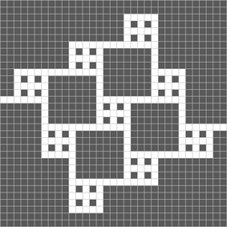
A path in the picture above is defined as a sequence of cells such that:

  • It begins on the leftmost white cell and ends on the rightmost white cell.
  • It only uses white cells.
  • Any two consecutive cells in the path are orthogonally adjacent (share a side).
  • Any two orthogonally adjacent cells appear consecutive in at most one position. (Essentially this means the path doesn't cross any side of any square more than once.) Note that a path may use a square more than once, only that it may not cross a side more than once.

If you're familiar with Path counting , this is pretty much the same definition of path as used in that problem, only made more formal.

In fact, the question is the same. Compute the number of possible paths in the picture above.


The answer is 104534074800.

This section requires Javascript.
You are seeing this because something didn't load right. We suggest you, (a) try refreshing the page, (b) enabling javascript if it is disabled on your browser and, finally, (c) loading the non-javascript version of this page . We're sorry about the hassle.

2 solutions

Ivan Koswara
Feb 20, 2015

The method of solving it is largely the same as in the first version, but now with more delicate counting.

Each small grid has five possible states:

  • Not passed at all
  • Passed from a corner to the opposite corner
  • Passed from a corner to an adjacent corner
  • Passed twice, in both cases to the opposite corner
  • Passed twice, in both cases to an adjacent corner

We then count each possible state carefully. In order given above, there are 1 , 16 , 15 , 2 , 9 1, 16, 15, 2, 9 possible ways respectively.

Now we look on each individual path of the second case. Why the second case? Because the large grid resembles exactly the second case, passing from a corner (left) to the opposite corner (right). Each of these sixteen paths correspond to the "large path" taken in the large grid, and will use the small grids in different ways, leaving them in different states. For example, consider the following path: down, right, right, up, left, down, down, right.

Considering only the states of the small grids, we can consider only this:

Thus our DRRULDDR path is essentially "1 none, 1 across, 6 adjacent, 1 twice across, 0 twice adjacent". That's all we need to consider.

Now, take a large path and consider the small grids. Suppose there are a , b , c , d , e a,b,c,d,e small grids of each state respectively. That is, a a small grids aren't used at all; b b small grids are traversed once, across; c c small grids are traversed once, to an adjacent corner; and so on. Then the corresponding number of actual path is simply 1 a 1 6 b 1 5 c 2 d 9 e 1^a \cdot 16^b \cdot 15^c \cdot 2^d \cdot 9^e . Our DRRULDDR example corresponds to 1 1 1 6 1 1 5 6 2 1 9 0 = 364500000 1^1 \cdot 16^1 \cdot 15^6 \cdot 2^1 \cdot 9^0 = 364500000 paths in total.

By computing each of the sixteen paths carefully, we arrive at the following ( a , b , c , d , e ) (a,b,c,d,e) values and thus the number of paths contributed:

  • RRDD: ( 4 , 3 , 2 , 0 , 0 ) = 921600 (4,3,2,0,0) = 921600
  • RDRD: ( 4 , 1 , 4 , 0 , 0 ) = 810000 (4,1,4,0,0) = 810000
  • RDDR: ( 4 , 3 , 2 , 0 , 0 ) = 921600 (4,3,2,0,0) = 921600
  • DRRD: ( 4 , 1 , 4 , 0 , 0 ) = 810000 (4,1,4,0,0) = 810000
  • DRDR: ( 4 , 1 , 4 , 0 , 0 ) = 810000 (4,1,4,0,0) = 810000
  • DDRR: ( 4 , 3 , 2 , 0 , 0 ) = 921600 (4,3,2,0,0) = 921600
  • RRDLDR: ( 2 , 3 , 4 , 0 , 0 ) = 207360000 (2,3,4,0,0) = 207360000
  • RDLDRR: ( 2 , 3 , 4 , 0 , 0 ) = 207360000 (2,3,4,0,0) = 207360000
  • DDRURD: ( 2 , 1 , 6 , 0 , 0 ) = 182250000 (2,1,6,0,0) = 182250000
  • DRURDD: ( 2 , 1 , 6 , 0 , 0 ) = 182250000 (2,1,6,0,0) = 182250000
  • RRDLLDRR: ( 0 , 5 , 4 , 0 , 0 ) = 53084160000 (0,5,4,0,0) = 53084160000
  • DDRUURDD: ( 0 , 3 , 6 , 0 , 0 ) = 46656000000 (0,3,6,0,0) = 46656000000
  • RDLDRURD: ( 1 , 1 , 6 , 0 , 1 ) = 1640250000 (1,1,6,0,1) = 1640250000
  • DRURDLDR: ( 1 , 1 , 6 , 0 , 1 ) = 1640250000 (1,1,6,0,1) = 1640250000
  • RDDLURRD: ( 1 , 1 , 6 , 1 , 0 ) = 364500000 (1,1,6,1,0) = 364500000
  • DRRULDDR: ( 1 , 1 , 6 , 1 , 0 ) = 364500000 (1,1,6,1,0) = 364500000

Adding all sixteen values, we obtain the answer 104534074800 \boxed{104534074800} .

Brian Chen
Feb 20, 2015

I'm bored enough to use Haskell today. It's still destructive in the ST monad, but whatever. Theoretically, this post is literate Haskell.

Boring imports.

> import Control.Monad
> import Control.Monad.ST
> import Data.Array.MArray
> import Data.Array.ST
> import qualified Data.Map as Map

Type plumbing, introducing our ugly graph representation using an unboxed mutable array of booleans indexed by point pairs:

> type Pt = (Int,Int)
> type Graph s = STUArray s (Pt,Pt) Bool

Mutation helpers:

> setEdge :: Graph s -> Pt -> Pt -> Bool -> ST s ()
> setEdge g i j b = do
>     writeArray g (i,j) b
>     writeArray g (j,i) b
> getEdge :: Graph s -> Pt -> Pt -> ST s Bool
> getEdge g i j = readArray g (i,j)
> initGraph :: ST s (Graph s)
> initGraph = do
>     g <- newArray (((0,0),(0,0)),((2,2),(2,2))) False
>     forM_ [0..2] $ \i -> forM_ [0..1] $ \j -> do
>         setEdge g (i,j) (i,j+1) True
>         setEdge g (j,i) (j+1,i) True
>     return g

And the core DFS. For reusability, we record the path traveled so far as a list of Pt s and take a callback in the ST monad to determine what integer to sum over the leaves of the search. This generality allows us to stack two DFSes that must use different edges neatly. (The returned result could easily be generalized to an arbitrary monoid and the type signature might even be more intuitive that way, but we don't really need that generality here.)

Note that the path traveled so far is stored in reverse order because prepending to linked lists is O(1) but appending is slow.

> type Callback s = [Pt] -> ST s Integer

> dfs :: Graph s -> [Pt] -> Pt -> Pt -> Callback s -> ST s Integer
> dfs g path cur tgt cb = do
>     r <- if cur == tgt then cb (cur:path) else return 0
>     vs <- filterM (getEdge g cur) (range ((0,0),(2,2)))
>     fmap ((r +) . sum) . forM vs $ \i -> do
>         setEdge g cur i False
>         x <- dfs g (cur:path) i tgt cb
>         setEdge g cur i True
>         return x

To solve the subproblems in the small 2x2 grids, though, we don't need fancy callbacks, so here's a quick properly-typed utility function that always returns 1. Using this, we'll sum 1 across each discovered path to make the DFS find the total number of paths.

> one :: Callback s
> one = const (return 1)

Number of paths traveling from one corner of a 2x2 grid to another that shares a side with the first corner:

> sidePaths :: Integer
> sidePaths = runST $ do g <- initGraph; dfs g [] (0,0) (0,2) one

Number of paths traveling from one corner of a 2x2 grid to the corner diagonally across from it:

> diagPaths :: Integer
> diagPaths = runST $ do g <- initGraph; dfs g [] (0,0) (2,2) one

Number of pairs of paths traveling from one corner of a 2x2 grid to another corner that shares a side, and then between the remaining two corners:

> sideSidePaths :: Integer
> sideSidePaths = runST $ do
>     g <- initGraph
>     dfs g [] (0,0) (0,2) (const $ dfs g [] (2,0) (2,2) one)

Number of pairs of paths traveling from one corner of a 2x2 grid to the corner diagonally across from it, and then between the remaining two corners:

> diagDiagPaths :: Integer
> diagDiagPaths = runST $ do
>     g <- initGraph
>     dfs g [] (0,0) (2,2) (const $ dfs g [] (0,2) (2,0) one)

These are all the subgrid numbers we need. Now we need to tabulate the different types of paths in the big grid and determine what type of path or paths it requires in each subgrid.

First, a data type for the orientation of edges between two subgrids, with sanity checks to defend against bugs:

> data Orient = Horiz | Vert deriving Eq
> orient :: Pt -> Pt -> Orient
> orient (r,c) (r',c') = case (abs (r' - r), abs (c' - c)) of
>     (1,0) -> Vert
>     (0,1) -> Horiz
>     _ -> error "orienting non-adjacent points"

The type of path or paths required in a subgrid are determined by the orientations of the edges before and after said path --- if they are the same, it's between corners diagonally across from each other; if they're different, it's between corners sharing a side --- which in turn is determined by the positions of the subgrid and the positions before and after it:

> data PathType = Side | Diag deriving Eq
> buildPathTypePair :: Pt -> Pt -> Pt -> (Pt, [PathType])
> buildPathTypePair u v w
>     | orient u v == orient v w = (v, [Diag])
>     | otherwise = (v, [Side])

We map a list of path-types to the precomputed number of paths or path pairs in subgrids:

> countSubgridPaths :: [PathType] -> Integer
> countSubgridPaths [Side] = sidePaths
> countSubgridPaths [Diag] = diagPaths
> countSubgridPaths [Side,Side] = sideSidePaths
> countSubgridPaths [Diag,Diag] = diagDiagPaths
> countSubgridPaths _ = error "impossible"

Now for each path in the big grid, we collect the path types for same subgrids together via a Map of lists (the only possible subgrid where this can happen is the middle one, but anyway) and then multiply across each subgrid to count the number of ways to choose subgrid paths to achieve a path in the big grid:

> countWays :: [Pt] -> Integer
> countWays vs = product . map countSubgridPaths . Map.elems . Map.fromListWith (++) $ zipWith3 buildPathTypePair vs (drop 1 vs) (drop 2 vs)

The solution is now found by calling our DFS with a callback using countWays, taking care to add imaginary starting and ending points in the big grid to provide the right edges at the beginning and end.

> solution :: Integer
> solution = runST $ do
>     g <- initGraph
>     dfs g [(0,-1)] (0,0) (2,2) (return . countWays . ((2,3):))
> main :: IO ()
> main = print solution

0 pending reports

×

Problem Loading...

Note Loading...

Set Loading...