Consider a uniform rod of length b . One half of this rod has a linear mass density of λ 1 = 9 while the other half has a linear mass density of λ 2 = 1 . The rod is initially placed horizontally in a smooth, fixed hemispherical bowl and the denser side is on the left. It is then released from rest at this initial position.
Find the time period (in seconds) of the rod's oscillations.
Note:
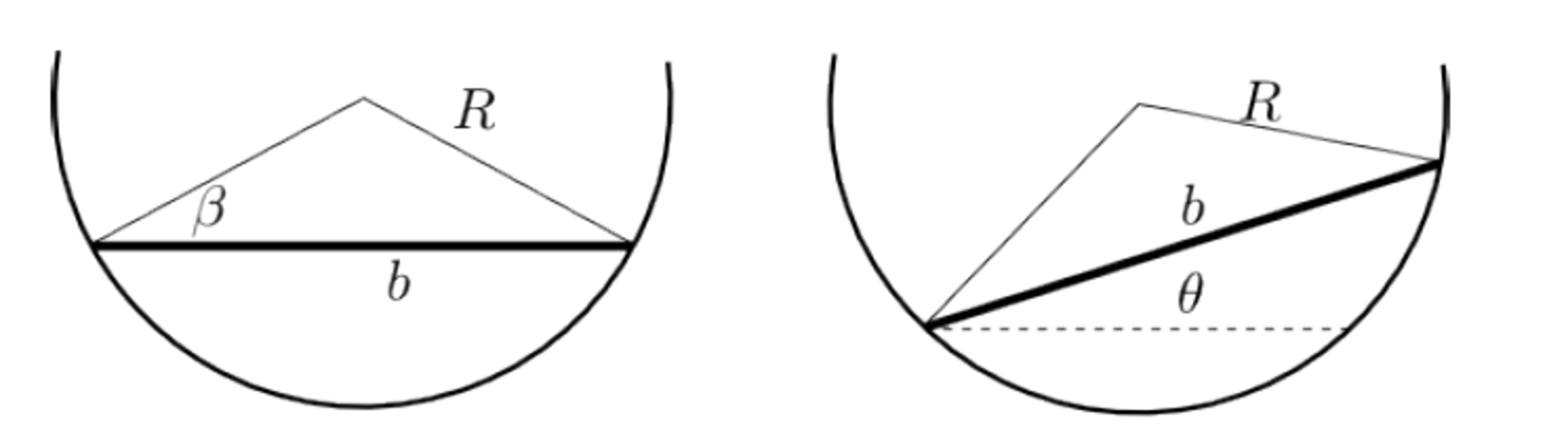
The diagram on the left shows the initial configuration while that on the right shows the configuration at an arbitrary instant of time.
Gravity ( g = 1 0 m / s 2 ) acts vertically downwards.
R = 2 m ; b = 0 . 5 m
β is the angle between the radius and the rod as shown in the figure.
Assume the absence of friction and other dissipative forces everywhere.
Hint:
This section requires Javascript.
You are seeing this because something didn't load right. We suggest you, (a) try
refreshing the page, (b) enabling javascript if it is disabled on your browser and,
finally, (c)
loading the
non-javascript version of this page
. We're sorry about the hassle.
@Karan Chatrath This was a fun series. Thanks for posting
Since total mechanical energy of the rod is constant, it's time derivative is zero. Simplifying this using the approximation for small angles the angle and it's sine are equal, we get the angular acceleration is negative, directly proportional to the angular displacement, with proportionality constant R 2 − 6 b 2 g R s i n β = 5 . 0 1 3 .
Therefore the time period is 5 . 0 1 3 2 π = 2 . 8 0 6
Thank you for sharing your approach. I like how you have used the total energy to derive the equation of motion. In my view, it is the fastest and easiest route to arrive at the equation of motion as opposed to Lagrangian mechanics and free body diagrams. However, in my view, I think it is missing a few steps. The rod is initially oriented at θ = 0 and it oscillates about its equilibrium position. So, by simply making a small angle approximation, you are linearising the equation about θ = 0 which is not the position about which the rod oscillates (mean position). I request you to refer to the other solution where a plot of θ vs. time is provided to see this behaviour which I have described. To analyse small oscillations, linearisation of the differential equation must take place about the equilibrium point. This point was calculated in a previous problem in which you have shared your solution. I will share an analytical solution to elaborate further when I can.
Log in to reply
I told about motion about the equilibrium configuration only. It's not the angle θ , but some constants added to it. The derivatives of the angle θ and the angular displacement from the equilibrium position are the same.
Problem Loading...
Note Loading...
Set Loading...
Building from the previous problem result, we have the following Lagrangian:
L = 2 5 b ( R 2 − 6 b 2 ) θ ˙ 2 − b g ( − 5 R sin ( θ + β ) + 2 3 b sin θ )
Equation of motion:
d t d ∂ θ ˙ ∂ L = ∂ θ ∂ L
Crunching this out results in:
5 b ( R 2 − 6 b 2 ) θ ¨ = − b g ( − 5 R cos ( θ + β ) + 2 3 b cos θ )
Numerically integrating results in a period of approximately 2 . 8 0 5 . The graph of θ vs. time is included below, along with the simulation code.