Potential Difference Over a Crazy Path
A force field is described as follows:
F = x + y r ^
This link goes to a Pastebin page where the ( x , y ) coordinates of the path C are listed. The points are listed sequentially. Define the potential difference:
Δ U = ∫ C F ⋅ d ℓ
Estimate the value of Δ U .
Details and Assumptions
1)
r
=
(
x
,
y
)
.
r
^
is a unit-length version of
r
2)
Microsoft Excel is a good tool for this problem, if you don't want to use a programming language
3)
The sign of
Δ
U
matters
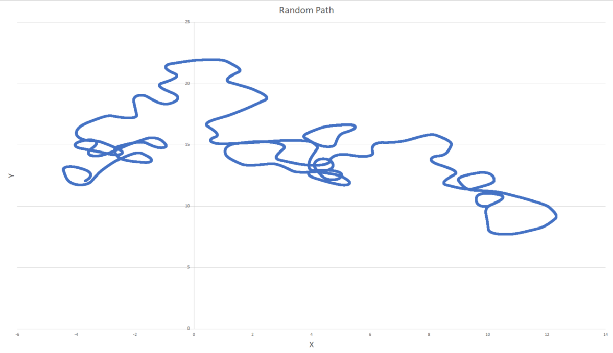
Bonus: Plot the path to visualize it. How would you generate a random smooth path such as this one?
The answer is -0.272.
This section requires Javascript.
You are seeing this because something didn't load right. We suggest you, (a) try
refreshing the page, (b) enabling javascript if it is disabled on your browser and,
finally, (c)
loading the
non-javascript version of this page
. We're sorry about the hassle.
2 solutions
Very nice! My thought was in the right direction then. Instead of thinking of a random differential equation which would be tedious, you apply a random force.
Log in to reply
Yeah, randomness is the essential element, but there are various ways of doing it. It's interesting to think that I can just suck up some electric energy and generate these things
Log in to reply
What's also interesting is that the electrical energy you used to perform these calculations is a consequence of the motion of electrons which are themselves tracing weird trajectories if somehow viewed at a subatomic scale.
Given:
F = ( x + y ) x 2 + y 2 x i ^ + ( x + y ) x 2 + y 2 y j ^ d l = d x i ^ + d y j ^
d ( Δ U ) = F ⋅ d l
Now, the numeric data is of length 10000. Let arbitrary index of the X-array and Y-array be denoted as k where k varies from 2 to 10000. F x ( k ) = ( x ( k ) + y ( k ) ) x ( k ) 2 + y ( k ) 2 x ( k ) F y ( k ) = ( x ( k ) + y ( k ) ) x ( k ) 2 + y ( k ) 2 y ( k ) d x ( k ) = x ( k ) − x ( k − 1 ) d y ( k ) = y ( k ) − y ( k − 1 ) d I ( k ) = F x ( k ) d x ( k ) + F x ( k ) d y ( k )
Add up all elements of the column d I to obtain the required answer of − 0 . 2 7 1 9 6 (work done using Excel). The path over which the integral is computed is as follows. To obtain a random path, I would just think of a random two-variable, time-varying (non-autonomous) and coupled non-linear system of differential equations (hopefully exhibiting chaotic behaviour) and solve them to obtain some arbitrary trajectory. But that thought process involves a bit of work. Is there a faster way?
Greetings! I was just wondering how you uploaded the array of data onto that paste-bin link. I was thinking of a problem involving a given dataset and this information would be helpful.
Log in to reply
Nevermind, I figured it out. Turns out I was pasting a very large volume of data because of which my browser kept crashing. Now I know better
@Karan Chatrath has provided a nice summary of how to solve this problem. I will describe the curve generation. My approach is to just apply a random force to a simulated particle and plot the particle trajectory. This code changes the force every second, and runs the simulation for 100 seconds. It also normalizes the speed to unity on every processing interval to prevent the particle from speeding up. It is somewhat amusing to generate these curves and plot them. Here is another random curve, as an example (not the same as the one from the problem)