Pulling with a Winch (Part 2)
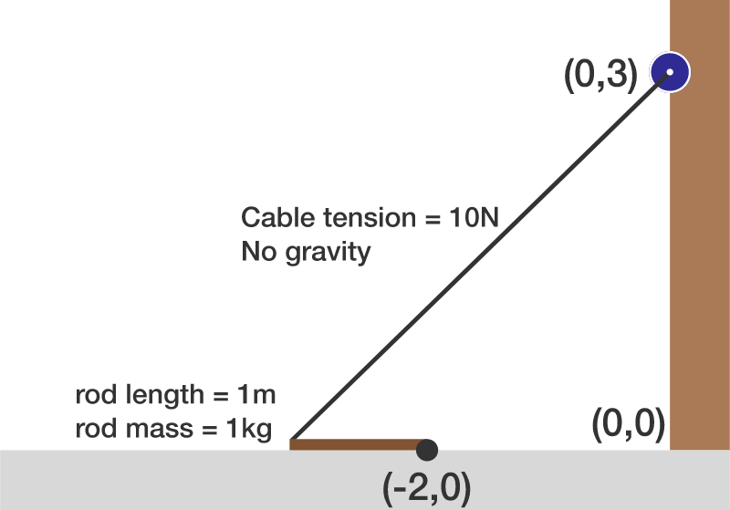
A winch located up a wall pulls on the free end of a rod whose other end is hinged to the floor. At the rod is horizontal and at rest, pointing away from the wall. The winch cable is kept under constant tension. Parameters are shown in the diagram. There is no gravity in this problem.
At what time (in seconds) does the rod become upright?
The answer is 0.36.
This section requires Javascript.
You are seeing this because something didn't load right. We suggest you, (a) try
refreshing the page, (b) enabling javascript if it is disabled on your browser and,
finally, (c)
loading the
non-javascript version of this page
. We're sorry about the hassle.
I hacked at this like an amateur, but I got there...mostly by luck.
Here is a diagram of my initial setup:
Then from Newton's Second Law around the hinge, ∑ T = I α
F sin β L = 3 1 M L 2 θ ¨
Then to get β in terms of θ use the Law of Sines:
1 3 sin β = x sin ( π − arctan 2 3 − θ ) ⇒ sin β = x 1 3 sin ( π − arctan 2 3 − θ )
Then just to clean it up: π − arctan 2 3 = ϕ
Now to get x in terms of θ using the Law of Cosines:
x 2 = ( 1 3 ) 2 + L 2 − 2 L 1 3 cos ( ϕ − θ ) ⇒ x = 1 3 + L 2 − 2 L 1 3 cos ( ϕ − θ )
Making the proper substitutions and rearranging the second order non-linear ODE is obtained:
θ ¨ = M L 3 1 3 F 1 3 + L 2 − 2 L 1 3 cos ( ϕ − θ ) sin ( ϕ − θ )
From this point I had to veer from formal technique ( I 'm sure some will greatly simplify and formalize the solution technique ). I plotted θ ¨ v s . θ , broke it into 0.1 radian sections and graphically linearized each portion ( Using Excel Linear Trendlines ) The result of that process is shown below.
From here it was a matter of solving a series of 16 linear second order linear ODE's of the form:
θ ¨ = A θ + B for which there are two solutions types,
C a s e 1 : A > 0
θ ( t ) = C 1 e A t + C 2 e − A t − A B
C a s e 2 : A < 0
θ ( t ) = C 1 cos ( A t ) + C 2 sin ( A t ) + A B
subject to the initial conditions θ ( t o ) = θ o , and θ ˙ ( t o ) = ω o . Then I graphically determined the time ( t f ) at the end of each interval using the outputs of each interval ( θ f , ω f , t f ) as the inputs for the following interval.
Here are few sample calculations ( performed in Mathcad), the last of which shows my final result of 0.3649 seconds.