Stasis with Unequal Rods
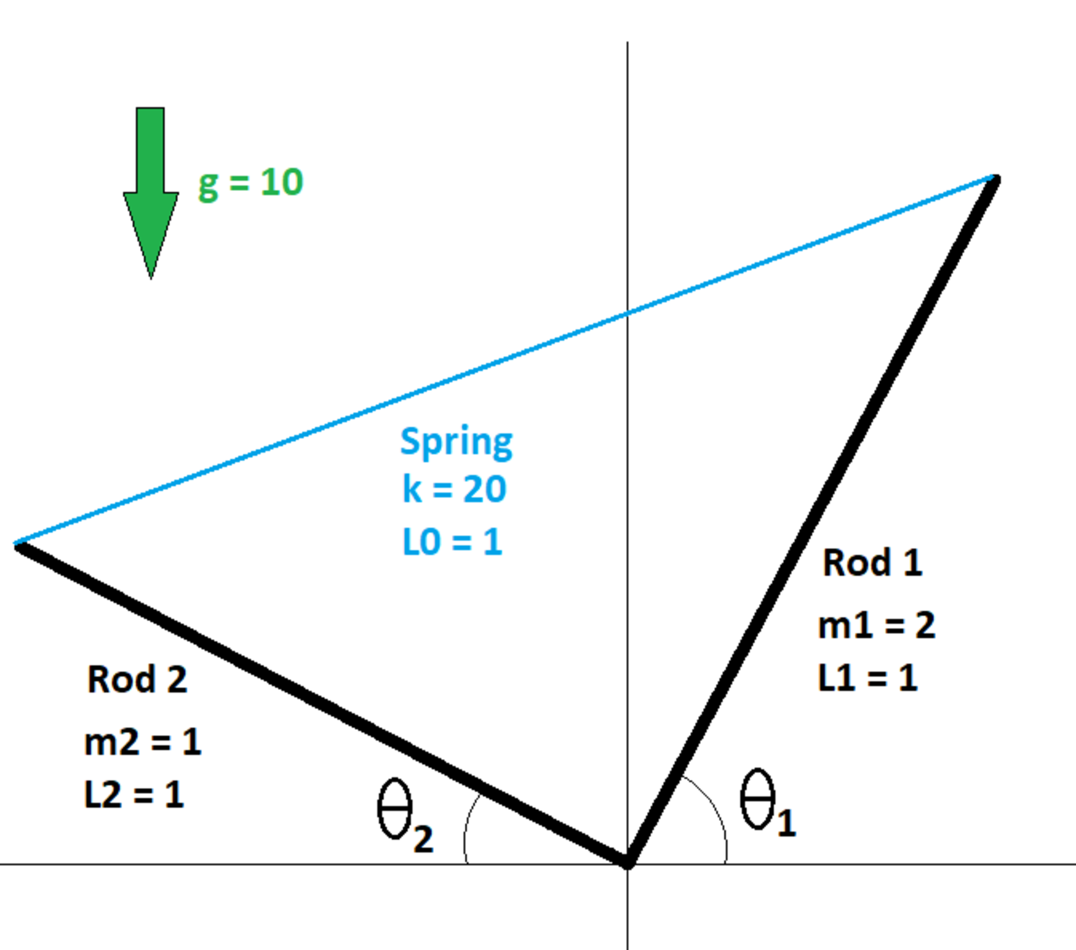
Two uniform rods are hinged about the origin. Each rod can rotate about the z axis independently of the other (the axis being perpendicular to the page). The other ends of both rods are connected by a spring. The diagram shows the masses and lengths of both rods, the force constant and natural length of the spring, and the ambient gravitational acceleration.
Given that angles θ 1 and θ 2 are in the range 0 < θ < 9 0 ∘ , and that the system is in stasis, determine angles θ 1 and θ 2 (in degrees). Give your answer as ⌊ 1 0 0 θ 1 ⌋ .
Bonus: There is another solution as well, that doesn't conform to the angle constraints given above. Can you find it?
The answer is 6605.
This section requires Javascript.
You are seeing this because something didn't load right. We suggest you, (a) try
refreshing the page, (b) enabling javascript if it is disabled on your browser and,
finally, (c)
loading the
non-javascript version of this page
. We're sorry about the hassle.
3 solutions
That's an interesting plot. Are there two potential minima? I have only found two solutions, so that's why I ask
Log in to reply
There are more than two minima. I found them by choosing random starting points in the Newton-Raphson iterations. Another configuration is when the rods are diametrically opposite and horizontal.
May I use the diagram in the problem statement for a follow-up problem? I have gone down a rabbit hole with this system and I want to draw attention to some details through a question.
Log in to reply
In the "A" equation, are the angular velocities in degrees per second or radians per second?
Most certainly. I look forward to it
I used energy approach mentioned by @Karan Chatrath which is very convenient in this case.
Physics says that equilibrium will occur once the potential energy of the system is minimal subject to the constraints. The rest of the problem is then of a mathematical kind. Here, it's obvious that there are two degrees of freedom, two independent coordinates - namely two angles. If we use l to denote the length of the spring, by cosine theorem we have: l 2 2 l ∂ θ i ∂ l = L 1 2 + L 2 2 − 2 L 1 L 2 cos ( π − θ 1 − θ 2 ) = L 1 2 + L 2 2 + 2 L 1 L 2 cos ( θ 1 + θ 2 ) = − 2 L 1 L 2 sin ( θ 1 + θ 2 ) , for i = 0 , 1 . Expression for potential energy is: U = 2 m 1 g L 1 sin θ 1 + 2 m 2 g L 2 sin θ 2 + 2 1 k ( l − L 0 ) 2 Equations are obtained by finding partial derivatives with respect to each coordinate and setting them to zero: ∂ θ i ∂ U = 2 m i g L i cos θ i + k ( l − L 0 ) ∂ θ i ∂ l = 2 m i g L i cos θ i − k L 1 L 2 sin ( θ 1 + θ 2 ) ( 1 − L 1 2 + L 2 2 + 2 L 1 L 2 cos ( θ 1 + θ 2 ) L 0 ) = 0 I used GeoGebra to plot these equations in θ 1 θ 2 -plane and find the intersection which satisfies given condition.
I used a hill-climbing algorithm which mutates the unknown angle parameters θ 1 and θ 2 until the net torque on each rod is zero. I have found the following solutions:
Solution 1
θ
1
≈
6
6
.
0
5
4
∘
θ
2
≈
3
5
.
7
3
3
∘
Solution 2
θ
1
≈
8
9
.
5
8
7
∘
θ
2
≈
−
8
9
.
1
7
5
∘
In the second solution, the two rods are nearly co-linear, almost lining up with the y axis. Also, the second and third decimal points in solution 2 are not as consistent as they are for solution 1.
1 2 3 4 5 6 7 8 9 10 11 12 13 14 15 16 17 18 19 20 21 22 23 24 25 26 27 28 29 30 31 32 33 34 35 36 37 38 39 40 41 42 43 44 45 46 47 48 49 50 51 52 53 54 55 56 57 58 59 60 61 62 63 64 65 66 67 68 69 70 71 72 73 74 75 76 77 78 79 80 81 82 83 84 85 86 87 88 89 90 91 92 93 94 95 96 97 98 99 |
|
For me, this was not an easy one to solve. In fact, I think there is a lot more to this problem than meets the eye. I will first present the solution that worked for me.
Notice how the spring and the two rods form a triangle. More specifically, an isosceles triangle. This is because of the rods having an equal length. From here, two equations can be formed by calculating the torque about the origin.
The angle between either rod and the spring is:
A = 2 θ 1 + θ 2
The above result follows from elementary geometry. Now the torque experienced by rod 1 about the origin is:
T 1 = 2 m 1 g L 1 cos θ 1 − F s L 1 sin A
The torque experienced by rod 2 about the origin is:
T 2 = 2 m 2 g L 2 cos θ 2 − F s L 2 sin A
Here,
F s = K ( ( cos θ 1 + cos θ 2 ) 2 + ( sin θ 2 − sin θ 1 ) 2 − 1 )
At equilibrium, the net torques experienced by each rod must be zero. The angles at which this occur can be found by writing a simple code which sweeps through the angles within the specified range. I have not attached the code here now. From there, the answer comes out to be:
θ 1 = 6 6 . 0 5 6 8 o
Hence the final answer is 6 6 0 5 .
Now, arriving at this answer took me more than one try. Whenever I encounter an equilibrium problem which involves no dissipative forces, my first instinct is to minimise the potential energy of the system.
The total potential energy of the system is the sum of gravitational potential energies of the rods and the energy stored in the spring.
V = 2 m 1 g L 1 sin θ 1 + 2 m 2 g L 2 sin θ 2 + 2 1 K ( ( cos θ 1 + cos θ 2 ) 2 + ( sin θ 2 − sin θ 1 ) 2 − 1 ) 2
Computing its gradient and equating it to zero (steps omitted here) would lead to a couple of nonlinear equations which would need to be solved numerically. I chose the Newton-Raphson method. The answer depends on the initial assumption. I was getting many weird equilibrium configurations but after some tries, found the required answer. Usually, the solution should be found with ease but that was not the case here. It involved quite a bit of work for me. And soon enough I realised why. The following 3D plot shows the variation of PE with the angles.
Given the odd shape of this surface, one can see that the required equilibrium point is definitely not stable. The odd shape also explains why the Newton Raphson iteration is so sensitive to the starting point.