To Iterate or Not to Iterate? (Part 2)

Calculus Level 5

$\large{x + e^{x}=0}$

Suppose that $x$ is a complex number in general, with a form $A+Bi$ (where $i=\sqrt{-1})$ .

Find the solution ( $x)$ to the above equation with the minimum value of $\sqrt{A^{2}+B^{2}}$ , subject to the constraint that $(B\not=0)$ .

Enter the corresponding value of $\sqrt{A^{2}+B^{2}}$ , to three decimal places.

The answer is 4.636.

2 solutions

Janardhanan Sivaramakrishnan
Sep 12, 2016

Use LambertW function.

$x+e^x=0 \implies 1=(-x)e^{-x}$

Therefore, $x=-W_n(1), n \in \mathbb{Z}$

The minimum magnitude non-real solution is $x=W_1(1)=1.534-4.375i$

Nice. I didn't know about this before. Thanks.

Steven Chase - 4 years, 9 months ago

Did your way, but in other way answer is wrong. Can you tell'em where it's wrong?

$x+e^x = 0 \\ \dfrac{d}{dx}(x + e^x) = \dfrac{d}{dx}0 \\ \dfrac{d}{dx}x + \dfrac{d}{dx}e^x = 0 \\ 1 + e^x = 0 \\ e^x + 1 = 0 \\ e^x + 1 = e^{i \pi} + 1 \\ e^x = e^{i \pi} \\ x = i \pi \\ A + iB = 0 + i\pi \\ A = 0, B = \pi \\ |x| = \sqrt[]{A^2 + B^2} = \sqrt[]{0 + \pi^2} = \pi \approx 3.1415$

Viki Zeta - 4 years, 9 months ago

The derivation is wrong. $f(x)=0$ implies $\frac{d}{dx}f(x)=0$ only if the first equation is satisfied for all values of $x$ .

A simple example :

$f(x)=x^2+3x+2=0$ and $\frac{d}{dx}f(x)=2x+3=0$ .

Solving the first equation gives $x=-1,-2$ and the second equation gives $x=-3/2$ .

In fact, the second equation gives the minimum/maximum/inflection in the graph of $f(x)$ .

Janardhanan Sivaramakrishnan - 4 years, 9 months ago

Steven Chase
Sep 11, 2016

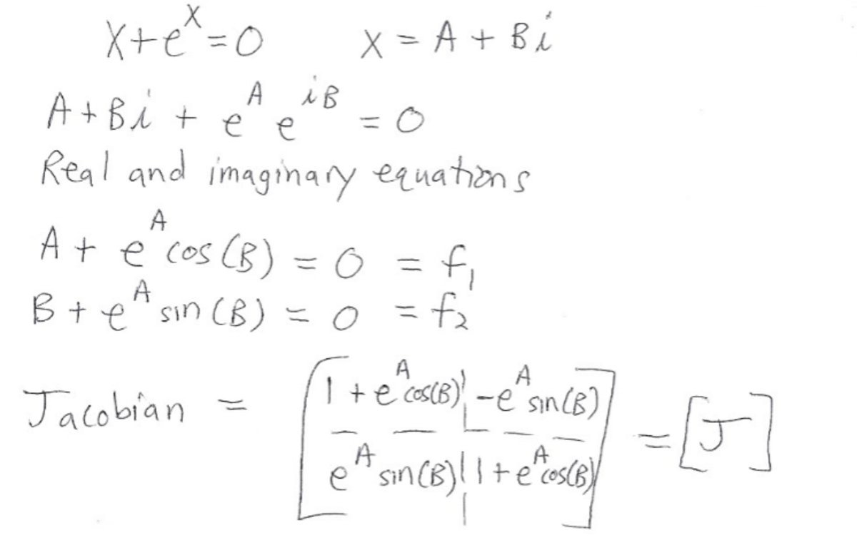
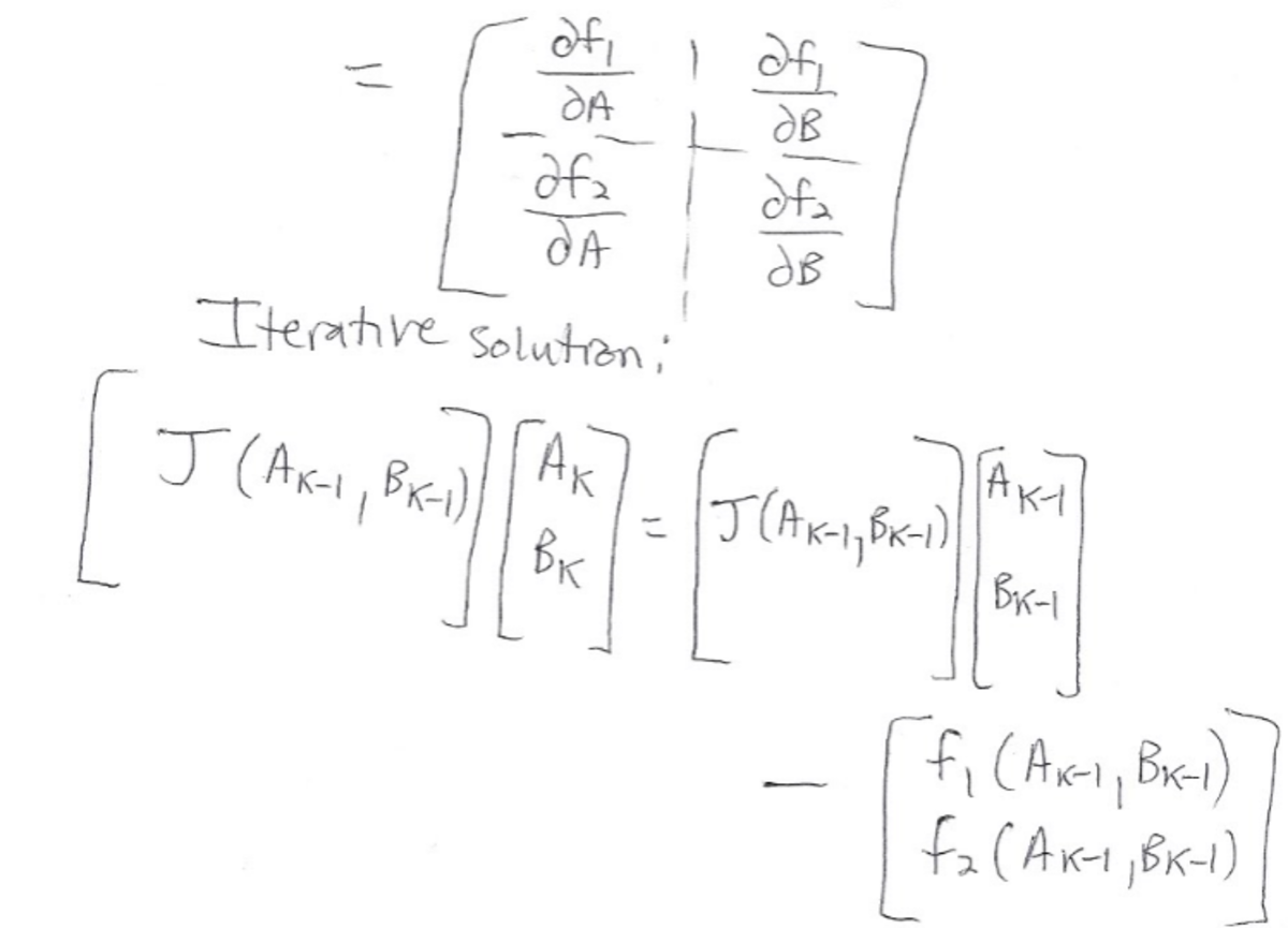
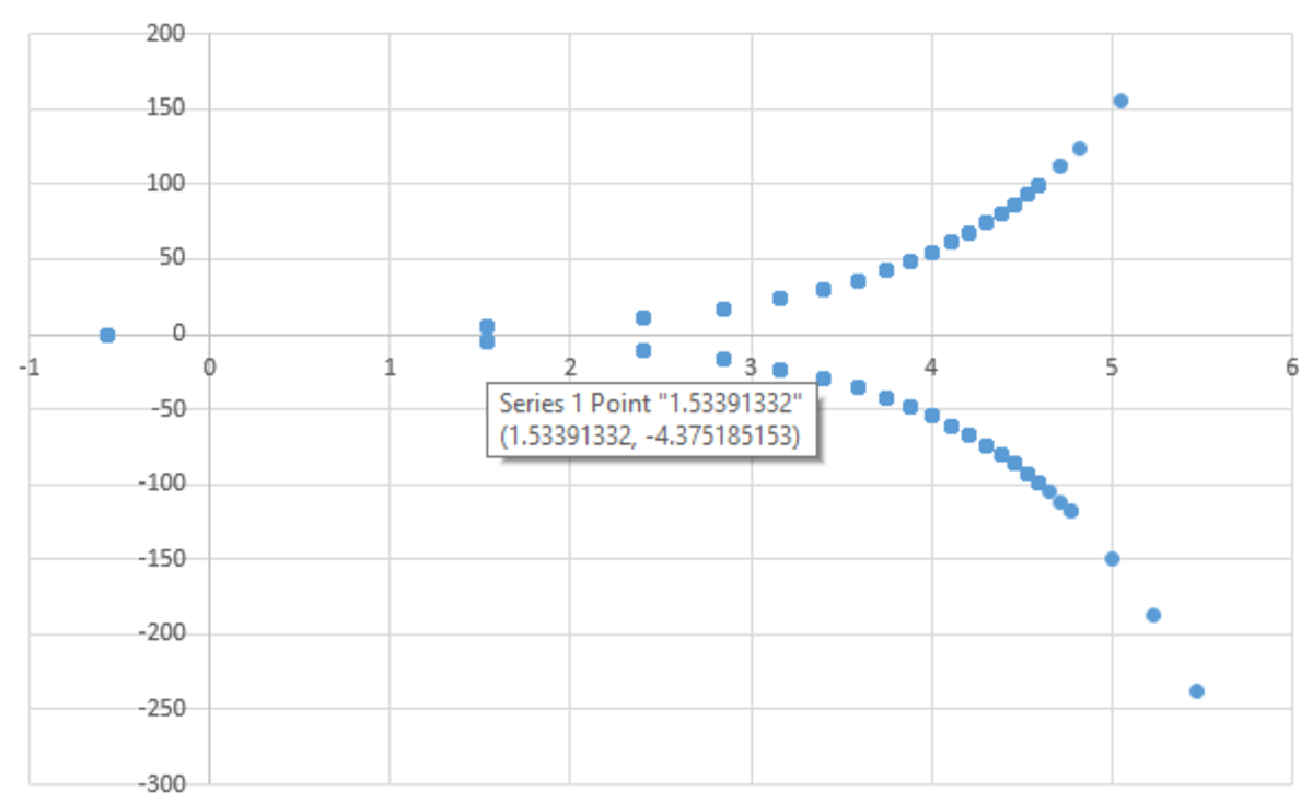
A good way to solve this is the multivariate Newton Raphson algorithm. Instead of taking a single derivative in one variable (see Newton Raphson page ), we use a matrix of partial derivatives, known as a Jacobian matrix. The analysis is shown below, as is a plot of some solutions in the complex plane. There is one real-valued solution, as well as a multitude of complex-valued solutions that are complex conjugates of each other. The complex solutions with the smallest value of $\sqrt{A^{2}+B^{2}}$ are 1.534 $\pm$ 4.375 $i$ , which each have a magnitude of about 4.636 . The solutions were generated by running the Newton Raphson algorithm many times with different randomized $(A,B)$ starting pairs. The particular random starting point determines which final solution the algorithm converges to. I have attached Python code for reference (this code can be put into a big loop and run many times to generate a plot). As a side note, hill-climbing algorithms and evolutionary algorithms are also good for solving these kinds of problems.

# Initial guesses

A = -100.0 + 200.0 * random.random()
B = -100.0 + 200.0 * random.random()


# Iterative solution


for j in range(0,100):

    f1 = A + math.exp(A)*math.cos(B)
    f2 = B + math.exp(A)*math.sin(B)


    fvec = np.array([f1,f2])

    J11 = 1.0 + math.exp(A) * math.cos(B)
    J12 = -math.exp(A) * math.sin(B)

    J21 = math.exp(A) * math.sin(B)
    J22 = 1.0 + math.exp(A) * math.cos(B)


    J =  np.array([[J11,J12],[J21,J22]])
    vec = np.array([A,B])

    right = np.dot(J,vec) - fvec


    Sol = np.linalg.solve(J, right)

    A = Sol[0]
    B = Sol[1]

f1 = A + math.exp(A)*math.cos(B)
f2 = B + math.exp(A)*math.sin(B)

res = math.fabs(f1) + math.fabs(f2)

if res <= 10.0**-4.0:

    print A,B

To Iterate or Not to Iterate? (Part 2)

The answer is 4.636.

2 solutions

0 pending reports