  1
  2
  3
  4
  5
  6
  7
  8
  9
 10
 11
 12
 13
 14
 15
 16
 17
 18
 19
 20
 21
 22
 23
 24
 25
 26
 27
 28
 29
 30
 31
 32
 33
 34
 35
 36
 37
 38
 39
 40
 41
 42
 43
 44
 45
 46
 47
 48
 49
 50
 51
 52
 53
 54
 55
 56
 57
 58
 59
 60
 61
 62
 63
 64
 65
 66
 67
 68
 69
 70
 71
 72
 73
 74
 75
 76
 77
 78
 79
 80
 81
 82
 83
 84
 85
 86
 87
 88
 89
 90
 91
 92
 93
 94
 95
 96
 97
 98
 99
100
101
102
103
104
105
106
107
108
109
110
111
112
113
114
115
116
117
118
119
120
121
122
123
124
125
126
127
128
129
130
131
132
133
134
135
136
137
138
139
140
141
142
143
144
145
146
147
148
149
150
151
152
153
154
155
156
157
158
159
160
161
162
163
164
165
166
167
168
169
170
171
172
173
174
175
176
177
178
179
180
181
182
183
184
185
186
187
188
189
190
191
192
193
194
195
196
197
198
199
200
201
202
203
204
205
206
207
208
209
210
211
212
213
214
215
216
217
218
219
220
221
222
223
224
225
226
227
228
229
230
231
232
233
234
235
236
237
238
239
240
241
242
243
244
245
246
247
248
249
250
251
252
253
254
255
256
257
258
259
260
261
262
263
264
265
266
267
268
269
270
271
272
273
274
275
276
277
278
279
280
281
282
283
284
285
286
287
288
289
290
291
292
293
294
295
296
297
298
299
300
301
302
303
304
305
306
307
308
309
310
311
312
313
314
315
316
317
318
319
320
321
322
323
324
325
326
327
328
329
330
331
332
333
334 | import math
import copy
numrev = 5 # Number of revolutions
numper = 36 # Number of frames per revolution
Rt = 1.0 # Toroid radius
Rcs = .3 # Toroid cross section
Nf = numrev * numper # Number of cross section frames
Ns = 8 # Number of sides for the cross section
thetat = 0.0 # Angle in the xy plane at which a cross sectional frame is located (toroid originally lies in the xy plane with z axis as the central axis)
dthetat = 2.0 * math.pi / numper # xy plane angular separation between cross sectional frames
thetacs = 0.0 # Angle for determinng cross section points
dthetacs = 2.0 * math.pi / Ns # Angular separation between the points in a cross section
disprotxy = (10.0 / 180.0) * math.pi # Rotation angle in the xy plane for display #10 is default
disprotxz = (40.0 / 180.0) * math.pi # Rotation angle in the xz plane for display # 40 is default
disprotyz = (50.0 / 180.0) * math.pi # Rotation angle in the yz plane for display # 50 is default
coord = [] # xyz coordinates of a point within the toroid / frame
frame = [] # Array containing coordinates for all points within a frame
toroid = [] # Array containing all frames within the toroid
points = [] # Master array of all points
block = [] # Blocking array
# Create the frames
# Initialize xyz coordinates
x = 0.0
y = 0.0
z = 0.0
for k in range(0,Nf): # For each frame
frame = []
for j in range(0,Ns): # Assign coordinates to every point within the frame and append to the frame array
coord = []
x = (Rt + Rcs * math.cos(thetacs))*math.cos(k*dthetat)
y = (Rt + Rcs * math.cos(thetacs))*math.sin(k*dthetat)
z = Rcs * math.sin(thetacs) + k * (3.0 * Rcs)/(numper)
coord.append(x)
coord.append(y)
coord.append(z)
frame.append(coord[:])
thetacs = thetacs + dthetacs
toroid.append(frame[:]) # Append first frame to the toroid array
# Apply display rotations to all points within the toroid
x = 0.0
y = 0.0
z = 0.0
Rxy = 0.0
thetaxy = 0.0
Rxz = 0.0
thetaxz = 0.0
Ryz = 0.0
thetayz = 0.0
for j in range(0,Nf): # For every frame
for k in range(0,Ns): # For every point
x = toroid[j][k][0]
y = toroid[j][k][1]
z = toroid[j][k][2]
Rxy = math.hypot(x,y)
thetaxy = math.atan2(y,x)
x = Rxy * math.cos(thetaxy + disprotxy)
y = Rxy * math.sin(thetaxy + disprotxy)
Rxz = math.hypot(x,z)
thetaxz = math.atan2(z,x)
x = Rxz * math.cos(thetaxz + disprotxz)
z = Rxz * math.sin(thetaxz + disprotxz)
Ryz = math.hypot(z,y)
thetayz = math.atan2(z,y)
y = Ryz * math.cos(thetayz + disprotyz)
z = Ryz * math.sin(thetayz + disprotyz)
toroid[j][k][0] = x
toroid[j][k][1] = y
toroid[j][k][2] = z
#print toroid[j][k][0],toroid[j][k][1],toroid[j][k][2]
# Form master point array
for j in range(0,Nf-1): # For every frame
for k in range(0,Ns): # For every point
xp = toroid[j][k][0]
yp = toroid[j][k][1]
zp = toroid[j][k][2]
diffx = (toroid[j][k-1][0] - xp) / 10.0
diffy = (toroid[j][k-1][1] - yp) / 10.0
diffz = (toroid[j][k-1][2] - zp) / 10.0
for m in range(0,10):
points.append([xp,yp,zp])
xp = xp + diffx
yp = yp + diffy
zp = zp + diffz
diffx = (toroid[j+1][k-1][0] - xp) / 10.0
diffy = (toroid[j+1][k-1][1] - yp) / 10.0
diffz = (toroid[j+1][k-1][2] - zp) / 10.0
for m in range(0,10):
points.append([xp,yp,zp])
xp = xp + diffx
yp = yp + diffy
zp = zp + diffz
diffx = (toroid[j+1][k][0] - xp) / 10.0
diffy = (toroid[j+1][k][1] - yp) / 10.0
diffz = (toroid[j+1][k][2] - zp) / 10.0
for m in range(0,10):
points.append([xp,yp,zp])
xp = xp + diffx
yp = yp + diffy
zp = zp + diffz
diffx = (toroid[j][k][0] - xp) / 10.0
diffy = (toroid[j][k][1] - yp) / 10.0
diffz = (toroid[j][k][2] - zp) / 10.0
for m in range(0,10):
points.append([xp,yp,zp])
xp = xp + diffx
yp = yp + diffy
zp = zp + diffz
#for j in range(0,len(points)):
#print points[j][0],points[j][1]
# Form blocking surfaces
for j in range(0,Nf-1): # For every frame
for k in range(0,Ns): # For every cross section point
block.append([[toroid[j][k][0],toroid[j][k][1],toroid[j][k][2]],[toroid[j][k-1][0],toroid[j][k-1][1],toroid[j][k-1][2]],[toroid[j+1][k][0],toroid[j+1][k][1],toroid[j+1][k][2]]])
block.append([[toroid[j+1][k-1][0],toroid[j+1][k-1][1],toroid[j+1][k-1][2]],[toroid[j][k-1][0],toroid[j][k-1][1],toroid[j][k-1][2]],[toroid[j+1][k][0],toroid[j+1][k][1],toroid[j+1][k][2]]])
Robs = 10.0
thetaobs = 0.0
phiobs = 0.0
screendist = 9.0
scsize = 1.0
screen = [[screendist,0.0,0.0],[math.hypot(scsize,screendist),math.atan2(scsize,screendist),0.0],[math.hypot(scsize,screendist),0.0,math.atan2(scsize,screendist)]]
nn = 50.0
dtheta = (nn * 7.2 / 180.0) * math.pi
dphi = (0.0 / 180.0) * math.pi
thetaobs = thetaobs + dtheta
screen[0][1] = screen[0][1] + dtheta
screen[1][1] = screen[1][1] + dtheta
screen[2][1] = screen[2][1] + dtheta
phiobs = phiobs + dphi
screen[0][2] = screen[0][2] + dphi
screen[1][2] = screen[1][2] + dphi
screen[2][2] = screen[2][2] + dphi
Ox = Robs * math.sin(thetaobs) * math.cos(phiobs)
Oy = Robs * math.sin(phiobs)
Oz = Robs * math.cos(thetaobs) * math.cos(phiobs)
dummy0 = screen[0][:]
dummy1 = screen[1][:]
dummy2 = screen[2][:]
screen[0][0] = dummy0[0] * math.sin(dummy0[1]) * math.cos(dummy0[2])
screen[0][1] = dummy0[0] * math.sin(dummy0[2])
screen[0][2] = dummy0[0] * math.cos(dummy0[1]) * math.cos(dummy0[2])
screen[1][0] = dummy1[0] * math.sin(dummy1[1]) * math.cos(dummy1[2])
screen[1][1] = dummy1[0] * math.sin(dummy1[2])
screen[1][2] = dummy1[0] * math.cos(dummy1[1]) * math.cos(dummy1[2])
screen[2][0] = dummy2[0] * math.sin(dummy2[1]) * math.cos(dummy2[2])
screen[2][1] = dummy2[0] * math.sin(dummy2[2])
screen[2][2] = dummy2[0] * math.cos(dummy2[1]) * math.cos(dummy2[2])
#print Ox,Oy,Oz
#print screen
for j in range(0,len(points)): # For every point
disp = 1
for m in range(0,len(block)): # Compare every point against each surface to find intersections
B1x = (block[m][1][0] - block[m][0][0])
B1y = (block[m][1][1] - block[m][0][1])
B1z = (block[m][1][2] - block[m][0][2])
B2x = (block[m][2][0] - block[m][0][0])
B2y = (block[m][2][1] - block[m][0][1])
B2z = (block[m][2][2] - block[m][0][2])
Nx = B1y * B2z - B2y * B1z
Ny = B2x * B1z - B1x * B2z
Nz = B1x * B2y - B2x * B1y
Px = points[j][0]
Py = points[j][1]
Pz = points[j][2]
Cx = block[m][0][0]
Cy = block[m][0][1]
Cz = block[m][0][2]
alpha = (Nx * (Cx - Px) + Ny * (Cy - Py) + Nz * (Cz - Pz)) / (Nx * (Ox - Px) + Ny * (Oy - Py) + Nz * (Oz - Pz))
if (alpha > 0.0) and (alpha <=1.0): # if the ray intersects the infinte planar region between P and O
Rx = Px + alpha * (Ox - Px)
Ry = Py + alpha * (Oy - Py)
Rz = Pz + alpha * (Oz - Pz)
vdeltax = Rx - Cx
vdeltay = Ry - Cy
vdeltaz = Rz - Cz
B1x = B1x + .000000001
B2y = B2y + .000000001
sigma = (vdeltay - (B1y * vdeltax) / B1x) / (B2y - (B1y * B2x) / B1x)
gamma = (vdeltax - sigma * B2x) / B1x
if (sigma > 0.0) and (gamma > 0.0) and (sigma + gamma < 1) and (alpha > .007): # if the ray intersects a surface, don't display
disp = 0
#print j,m
if disp == 1:
B1x = (screen[1][0] - screen[0][0]) / scsize
B1y = (screen[1][1] - screen[0][1]) / scsize
B1z = (screen[1][2] - screen[0][2]) / scsize
B2x = (screen[2][0] - screen[0][0]) / scsize
B2y = (screen[2][1] - screen[0][1]) / scsize
B2z = (screen[2][2] - screen[0][2]) / scsize
#print B1x,B1y,B1z,B2x,B2y,B2z
Nx = B1y * B2z - B2y * B1z
Ny = B2x * B1z - B1x * B2z
Nz = B1x * B2y - B2x * B1y
#print Nx,Ny,Nz
Px = points[j][0]
Py = points[j][1]
Pz = points[j][2]
Cx = screen[0][0]
Cy = screen[0][1]
Cz = screen[0][2]
#print Cx,Cy,Cz
alpha = (Nx * (Cx - Px) + Ny * (Cy - Py) + Nz * (Cz - Pz)) / (Nx * (Ox - Px) + Ny * (Oy - Py) + Nz * (Oz - Pz))
#print alpha
Rx = Px + alpha * (Ox - Px)
Ry = Py + alpha * (Oy - Py)
Rz = Pz + alpha * (Oz - Pz)
vdeltax = Rx - Cx
vdeltay = Ry - Cy
vdeltaz = Rz - Cz
#print vdeltax,vdeltay,vdeltaz
B1x = B1x + .000000001
B2y = B2y + .000000001
sigma = (vdeltay - (B1y * vdeltax) / B1x) / (B2y - (B1y * B2x) / B1x)
gamma = (vdeltax - sigma * B2x) / B1x
if math.fabs(sigma) < scsize and math.fabs(gamma) < scsize:
print gamma,sigma
|
Easy Math Editor
This discussion board is a place to discuss our Daily Challenges and the math and science related to those challenges. Explanations are more than just a solution — they should explain the steps and thinking strategies that you used to obtain the solution. Comments should further the discussion of math and science.
When posting on Brilliant:
*italics*or_italics_**bold**or__bold__paragraph 1
paragraph 2
[example link](https://brilliant.org)> This is a quote# I indented these lines # 4 spaces, and now they show # up as a code block. print "hello world"\(...\)or\[...\]to ensure proper formatting.2 \times 32^{34}a_{i-1}\frac{2}{3}\sqrt{2}\sum_{i=1}^3\sin \theta\boxed{123}Comments
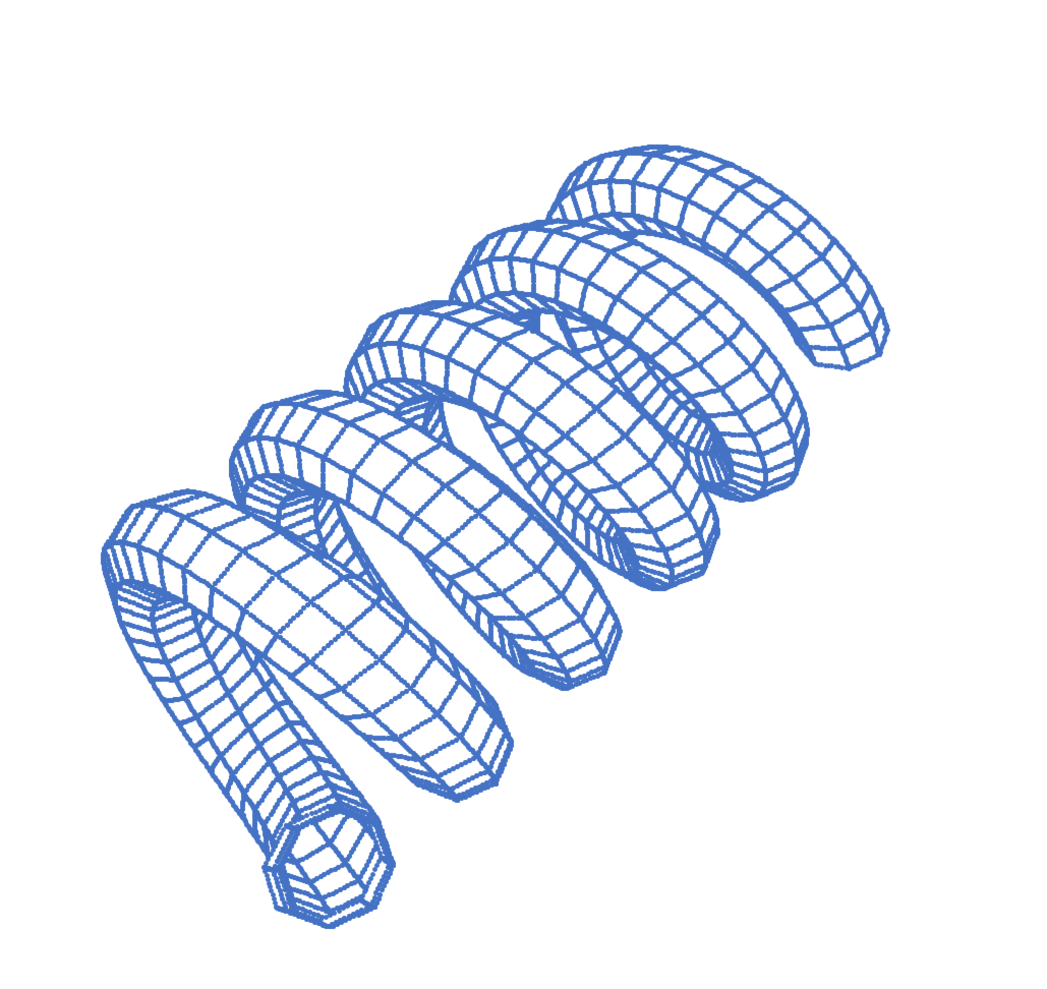
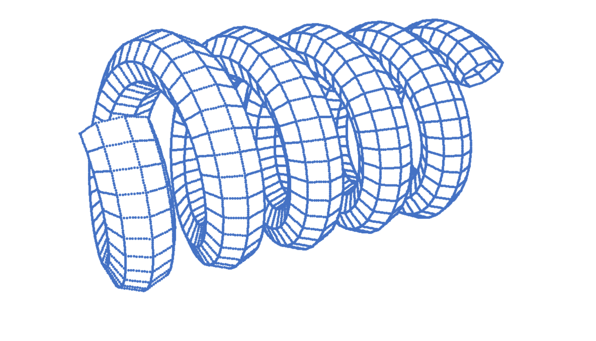
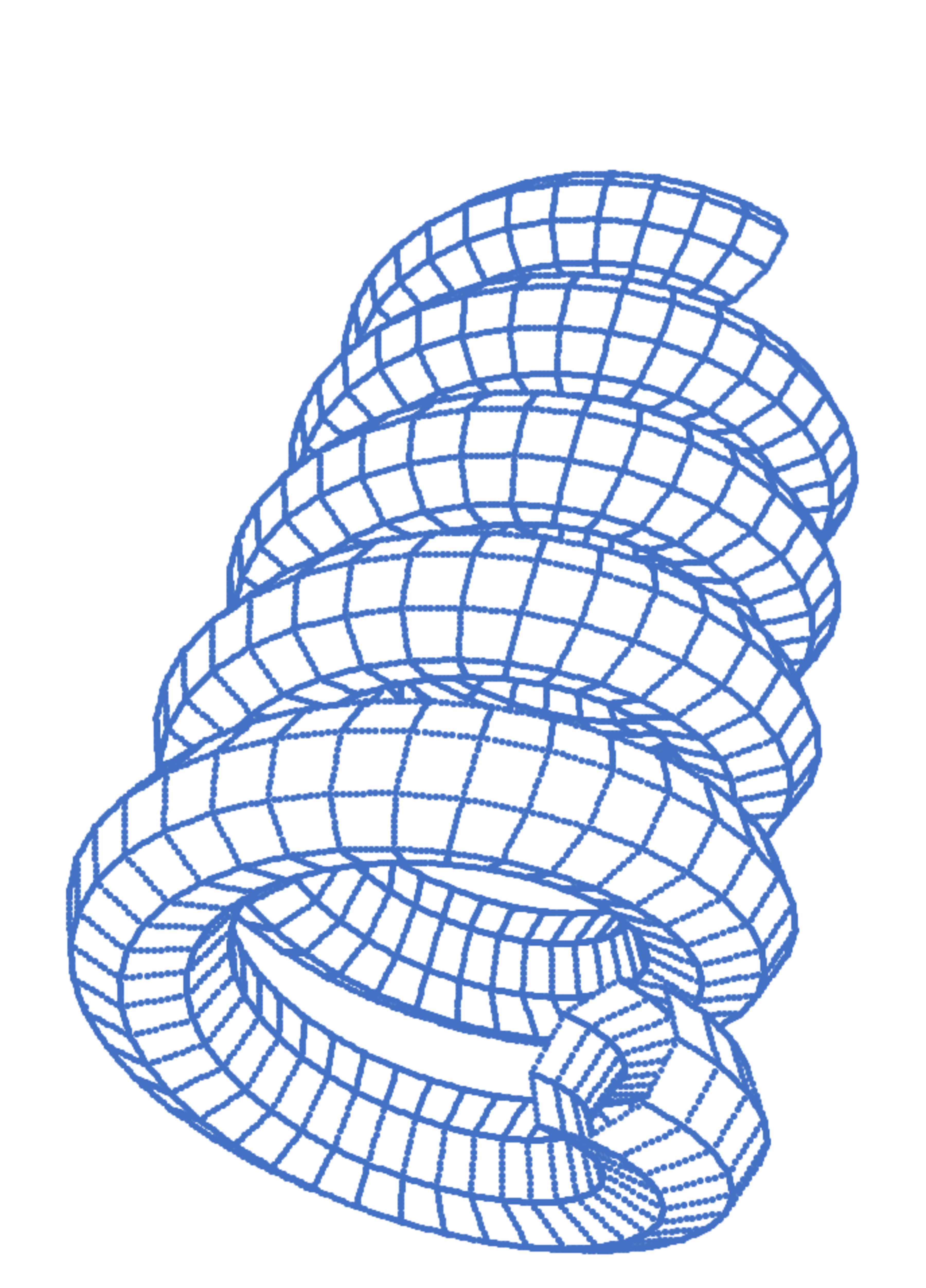
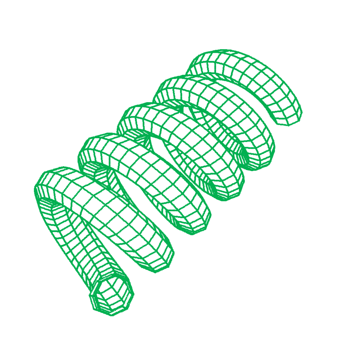
@Neeraj Anand Badgujar Here it is, as requested
@Karan Chatrath In case you are interested
Log in to reply
@Steven Chase VERYBEAUTIFUL I was thinking that this profile image you have taken from somewhere but after seeing this I realized that it is made by you only.
@Steven Chase in your profile the image is of light blue colour. Can you please give me the image in green colour.
Log in to reply
I have added a green version
Log in to reply
@Steven Chase This Images are very nice. Thanks for the green version.
Log in to reply
You're welcome. Glad you like them
Log in to reply
@Steven Chase yesterday in evening when I shared these images to my friends ,they were gone mad. But they don't use brilliant. They said me to say Thanks to the creator of this images. So, Thank you. Can you upload more image like this now.
@Steven Chase Sir in phython programming we can make this types of good images which we can't get in the web. Beside this image . Is there any more crazy images. I like this types of physics crazy images.
Log in to reply
Yeah, I have some more. I'll post those later as well
@Steven Chase Sir can you add YellowOrange and Red ? Please
Thank you for sharing this code. These graphics are pretty impressive considering you used just a python script to generate them. As for my profile picture, I just plotted two solutions of the Lorenz equations one over another in a dark background.
I will take a closer look at the code a little later as there seems to be a lot to unpack there. Pretty sure I'll learn something new in the process.
Nice image! I would personally do it using WebGL or OpenGL. Most of your graphics code in python would run on the CPU, so I think it would be a rather slow render for accuracy. That way GLSL is much faster as it makes use of the GPU. Very cool! I love python so much... I should learn CUDA python sometime. Maybe you should find the points using CUDA and then paste it into Microsoft Excel.
Log in to reply
Yeah, this program takes a ridiculously long time to run, but I've got time, so it's OK. Does the CUDA processing improve speed for serial algorithms, or only for parallel ones?
Log in to reply
You can parallelise the algorithm by coding a "kernel", so the computation will be much, much faster when all are computed simultaneously. I have been using computational methods to solve your problems recently. Same thing I noticed with the question "Curly Trajectory"; my code based on Euler Integration took a whopping 2 minutes to compile. CPU based
If you use GLSL and WebGL, and you can compute all the data points and store them in the vertex buffer in a parallel manner without going through the details of how OpenGL does that on your GPU.
It's so cool because there are in built functions in WebGL which can allow you to achieve the wireframe. You can do it without CUDA, because anyway you are producing a graphical output, which OpenGL excels at. What you have done in your python code would be done by C or C++, when defining the rasterisation and painting of the pixels in high resolution by WebGL. You've put together a very clever piece of code! You've done it from scratch. Well done man!
By the way, what are the specs of your PC?
@Steven Chase Just came here to see this beautiful images last time.
When you are going to share the files of your solutions and problems?
Do you find an alternative approach to share files ??