Lectures on Quantum Mechanics 2: The Schrödinger Equation

From Wave to Particle

Louis de Broglie taught us that all particles in the universe possess a wavelength. We will consider microscopic objects because they closely follow the wave-particle duality more than macroscopic objects. Consider a particle travelling in space with no potential holding it down: we will call this the free particle. Since microscopic particles also behave as a wave, we will model the free particle as a plane wave enveloped in a corresponding wave-packet. The plane wave propagates in space and evolves in time: $\Psi (x,t) = {e}^{i(kx-\omega t)}$ with a corresponding wave-packet: $\Psi(x,t) = \frac{1}{\sqrt{2\pi}}\int_{-\infty}^{\infty}{\phi(k)}{e}^{i(kx-\omega t) }dk.$

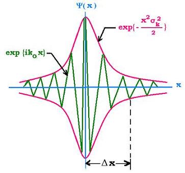Wave packet

Using de Broglie’s equations of momentum $p=\hbar k=\frac{h}{\nu}$ and energy $E= \hbar \omega = \frac{{p}^{2}}{2m}$ we can rewrite the wave-packet equation as $\Psi(x,t) = \frac{1}{\sqrt{2\pi \hbar}}\int_{-\infty}^{\infty}{\phi(p)}{e}^{i(px-Et)/ \hbar}dp.$

What can we do with this integral so that we can describe a physical system? Why not take derivatives until two sides of an equation match? Let’s begin by taking the time derivative and two derivatives in space: $\frac { \partial \Psi }{ \partial t } =\frac { 1 }{ \sqrt { 2\pi \hbar } } \int _{ -\infty }^{ \infty }{ \phi (p){ \left( \frac { -iE }{ \hbar } \right) e }^{ i(px-Et)/\hbar }dp }$

$\frac { \partial \Psi }{ \partial x } =\frac { 1 }{ \sqrt { 2\pi \hbar } } \int _{ -\infty }^{ \infty }{ \phi (p){ \left( \frac { ip }{ \hbar } \right) e }^{ i(px-Et)/\hbar }dp }$

$\frac { { \partial }^{ 2 }\Psi }{ \partial { x }^{ 2 } } =\frac { 1 }{ \sqrt { 2\pi \hbar } } \int _{ -\infty }^{ \infty }{ \phi (p){ \left( \frac { -{ p }^{ 2 } }{ { \hbar }^{ 2 } } \right) e }^{ i(px-Et)/\hbar }dp }.$

Now there is one final step to do: balancing. If we multiply the time derivative by $i\hbar$ and the second spatial derivative by $\frac{-{\hbar}^{2}}{2m}$, we get

$i\hbar \frac { \partial \Psi }{ \partial t } = \frac{-{\hbar}^{2}}{2m}\frac { { \partial }^{ 2 }\Psi }{ \partial { x }^{ 2 } }$

(this can be easily verified using the de Broglie equations).

It is customary in physics to describe physical systems in terms of total energy, which is the sum of the kinetic and potential energies. So all we have to do to this free particle is add $V\Psi$ to the right hand side. Hence,

$i\hbar \frac { \partial \Psi }{ \partial t } = \frac{-{\hbar}^{2}}{2m}\frac { { \partial }^{ 2 }\Psi }{ \partial { x }^{ 2 } }+ V\Psi.$

Operators

Quantum mechanics is inherently linear, which means linear algebra (more specifically linear operator algebra) is the language of QM. Thus, it is most appropriate to write the Schrödinger equation in operator form.

An operator is an instruction that is acted on a function. An operator $\hat{A}$ is linear if it satisfies the identity $\hat{A}[af(x)+bg(x)] = a\hat{A}f(x)+b\hat{A}g(x)$where $a,b$ are scalars. This is where QM starts to get abstract, so I will introduce some concrete examples. Consider the operators $\hat{p}=-i\hbar \frac{\partial}{\partial x}$ and $\hat{x}=x$ If we act $\hat{p}$ on some position quantity $x$, we get the differential $-i\hbar \frac{\partial x}{\partial x} = -i\hbar.$ Hence, momentum is a differential operator. Looks straightforward enough! But consider what we can do to operators ${\hat{p}}^{2} = {\left(-i\hbar \frac{\partial}{\partial x}\right)}^{2}$

${\hat{p}}^{2}= -{\hbar}^{2} \frac{{\partial}^{2}}{\partial {x}^{2}}$ which is convenient. Now let us look at the Schrödinger equation again…in operator form

$i\hbar \frac { \partial \Psi }{ \partial t } =\left[\frac{{\hat{p}}^{2}}{2m}+ \hat{V} \right] \Psi .$

For the time-independent case , we replace the time derivative term with total energy, and if we want to be even more compact, we may denote the operator on the right hand side with the Hamiltonian operator $\hat{H} = \hat{T} +\hat{V}$.

$E\Psi=\hat{H} \Psi .$

Notice how this is shorter? Well, that's good and all, but not the point. The point is that we are acting a Hamiltonian operator on the wavefunction $\Psi$, which is convenient for reasons unclear at the moment. You see, linear operators can describe many things, but all linear operators follow the same algebra. We have entered the realm where abstract algebra infiltrates all of physics for the convenience of problem solving. So from now on, we consider operators to act on physical quantities and objects.

Determinate States

When you solve the time-independent Schrödinger equation, you will encounter values of energy that satisfy $E\Psi=\hat{H} \Psi.$

These are called determinate states, which are eigenfunctions (also called eigenstates) of the linear operator $\hat{H}$ with corresponding energy eigenvalues $E$. When a linear operator possess several eigenvalues, we call the set of eigenvalues its spectrum. If two or more linearly independent eigenfunctions share the same eigenvalue, we call those spectra degenerate. You will later learn that degeneracies play an important role in describing the atom; hence much of quantum chemistry and solid-state physics. But for starters, you should solve the 1D particle in a box (Problem 3) below and calculate the corresponding energy eigenvalues ${E}_{n}$.

Visit my set Lectures on Quantum Mechanics for more notes.

Problems

1. Use the de Broglie relations to obtain the dispersion relation of wave-packets. Hint: $\omega \propto {k}^{2}$

2. 1D Particle in a Box Consider the potential that is 0 within the region $0<x<a$ and infinite elsewhere. Solve the time-independent Schrödinger equation for this potential with boundary conditions: $\Psi(0,t) = \Psi(a,t) = 0$ . Once you find the wavefunction (solution), normalize the wavefunction $\Psi(x,0)$.

   Note: $\Psi(x,t)$ is just $\Psi(x,0) {e}^{-iE t/\hbar}$

3. Now that you found the solution to the 1D Particle in a Box, find the set permissible eigenenergies (energy levels). Remember that the wavenumber of a matter-wave is given by $k=\frac{n\pi}{a}$ where $n=1,2,3,...$. This will help you simplify ${E}_{n}$.