On Shortest Path Algorithms in a Distributed Environment
You want to go from your home to to a gorgeous hike in the mountains. It is a beautiful day, and you want to to get to the trailhead as fast as you can, so you maximize your time on the trail. You get out a map and you find the shortest route to your destination.
Finding shortest paths in graphs is a fundamental problem in computer science. You are given a graph with some vertices (the locations in the map) and edges (roads in the map). The edges have associated weights (the distance along the edge, or the time it takes to traverse the edge.) With this input, you want to find a path from your beginning location to your destination with the minimum value of the sum of weights along it. A naive approach might be to examine all possible paths, but when the graph is large, there are far too many paths and this is very inefficient.
Correct!
27% of people got this right.
Consider an grid. (A 4 4 grid is shown below)
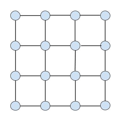
How many paths are there from the top left corner to the bottom right corner?
(Recall that a path in a graph is a sequence of distinct vertices in the graph such that consecutive pairs of vertices are connected by edges from the graph.)
Note: There is no restriction about only moving right or down. You can move in any direction.
Instead, a simple approach to finding the shortest path from a source to a destination is to start at the source and gradually grow a tree from the source. As you explore further and further outward, the tree is updated, so that at the end of the algorithm you have a "shortest path tree" (SPT) which is a tree such that for any vertex, the (unique) path through the tree from the root to that vertex is the shortest path in the original graph.
OK, that was pretty vague, because I did not tell you how to explore, nor how to do the updates. Nevertheless, when one has prescribed all the details, this is indeed the approach followed in Breadth First Search (where all the weights are 1), Dijkstra's Algorithm and the Bellman Ford Algorithm.
I am not going to go into the details of these algorithms here (that is already done in the wiki pages) but I will give a quick description of each one.
Breadth First Search Here we have a "current vertex", (initially the root), whose distance from the root is known. We grow the tree by marking all the neighbors of the current vertex which do not already know their distance to the root as being one step further from the root than the current vertex. Then we put these at the end of a queue of discovered vertices and take the front vertex from the queue to be the next "current vertex". The algorithm ends when the queue is empty.
Dijkstra's Algorithm Here we maintain a "current vertex", a partial SPT, and a "frontier". Initially, the current vertex and the partial SPT are both just the root, and the frontier is all the neighbors of the root, labelled with their distance from the root (the weight on the edge from the root) and pointing to the root as their parent in the tree. At each step of the algorithm, we select the "best vertex" from the frontier, i.e the one with the shortest distance to the root, to be the new current vertex, and add it to the partial SPT (it already has a proposed parent in the tree. Then we update the frontier by examining the neighbors of the current vertex and adding them to the frontier if they weren't already there (along with a tentative distance to the root and the current vertex as their tentative parent) or, if a neighbor was already in the frontier, it is updated with a new distance and parent if its distance to the root through the current vertex is less than its existing tentative distance (if not, then it is left alone). The algorithm ends when the frontier has been emptied out. The selection of the best vertex from the frontier is often done with a priority queue, although this was not the case in Dijkstra's original algorithm. One important requirement is that the weights are non-negative.
Bellman Ford Algorithm. Here, we maintain tentative distances to the root for all vertices. These start at infinity for all vertices other than the root itself (which naturally starts at 0.) At each stage of the algorithm, we examine all the edges, and if traversing an edge results in a lower distance to the root for one of its endpoints then the tentative distance of that endpoint is updated. The algorithm runs for such rounds where is the number of vertices.
So what are the differences in these algorithms, and how can one decide which one to pick for a particular application?
One answer is the kinds of weights. BFS is only applicable when all the weights are 1. When this is not the case, we must use one of the others. Dijkstra is only applicable when the weights are non-negative, so if there are negative weights, the only choice is to use Bellman Ford.
Another answer is run-time. In the case of non-negative weights either Dijkstra or Bellman Ford could be used. However, Dijkstra is much faster, with a run time of compared with . Here and are the sized of the vertex and edge sets respectively.
I want to offer another perspective, for why one may sometimes prefer the Bellman Ford algorithm over Dijkstra's algorithm, even when there are no negative weights.
How do we normally view running an algorithm? We are given some input (in the case of the shortest path problem, a weighted graph) and we have some code that implements the algorithm, that runs on a computer. We feed the input to the code, it processes it and (assuming it is correct) outputs the answer.
Now let us consider the following scenario. We have a very large graph with billions of vertices. At each vertex is a processor (aka computer). Some of the vertices are connected by cables, so that the processors at the vertices have the ability to communicate with each other. Sound familiar? (Did you say "the INTERNET?") So what happens when we want to communicate between processors that are not directly connected? We need to solve a routing problem. Of course, when you are really talking about the internet, you probably want shortest paths between all (or lots of) pairs of vertices, rather than single source shortest paths, but we will ignore that here.
So let us abstract away from that specific example. We have a graph with some vertices and some edges. At each vertex there is a processor. The collection of all these processors is our "computer", but at the same time, at least insofar as we want to solve the shortest path problem, the graph, that is the configuration of the various processors is also the input. So the computer acts on itself as input.
Now suppose we want to run a single-source shortest path algorithm on the graph, where the edge weights are the time taken to communicate along each cable. What happens if we try to run Dijkstra's algorithm? Look at it from the perspective of a single processor sitting at its vertex. This processor knows who its neighbors are, and whether or not it is the source vertex. If it is the source vertex, it can just advertise its existence to its neighbors, along with time stamps, and the neighbors can figure out how far they are from it (along a direct edge). What about a processor that knows it is not the root? Well, at least until it is discovered an put in the frontier, it has nothing to do except set infinity as its tentative distance to the source, and wait. But at some point it gets into the frontier, and realizes that its distance to the root is (say) 115 units. Great! Is that good because everybody else is at least 1000 units away? Or is it not so good because some other node is only 3 units away? The processor has no way of knowing what all the other tentative distances in the frontier are. At least, not without a lot of communication between them, and since the whole point of running a shortest path algorithm was to establish communication routes, we have a problem. The "greedy step" of Dijkstra's algorithm, where we decide which vertex is the next to be added to the tree is something that is fundamentally "non-local". It requires looking at the whole state of the computation, from the outside.
But wait a minute, you say. All the vertices in the frontier have some path to the root, even if it isn't the shortest. So they could just transmit their tentative distances to the root, and the processor at the root can select the best and let everyone know. Yes. This would work. But it is bad, for two reasons. One is that if we simply have the root do all the computation, and use the other nodes just as message relayers, then we have defeated the purpose of having a "computer" made up of several networked processors. We are wasting the computational power of all the other processors. The other reason is that relaying messages is generally considered to be more expensive than computational steps on an individual processor (aka local computation). Indeed, so great is the disparity that often abstract models of "Distributed Computation" simply allow you to do local computation for free, and measure the efficiency of an algorithm purely in terms of the number of sequential messages sent. Thus, implementing Dijkstra's algorithm in the described fashion is bad because it is preferring to send messages rather than try to compute as much as possible locally, but also compounding the problem because these messages are not even being sent along shortest paths. So we have destroyed the main advantage of Dijkstra's algorithm, which was its speed.
Not let us look at the Bellman Ford algorithm in the same context. Here, there is no greedy step. Each processor, sitting at its node starts out by setting its tentative distance to the root to be infinite (unless it is the source, in which case it sets it to 0). Then, on each round of the algorithm, it communicates with each of its neighbors, and tells them its own current tentative distance from the root, and receives the same data from its neighbors. If any of these communications results in its realizing it is closer to the root than it previously thought, then it updates its distance estimate. This happens for the prescribed number of rounds. (Let's assume for convenience that we know how many nodes are in the network). At no point in the algorithm did the processor need to know anything about distant nodes. Even though the algorithm as a whole examines all the edges each round, each individual processor only examines the edges to which it is immediately adjacent. Thus, the Bellman Ford algorithm is inherently local, or as it is sometimes called, "decentralized". No wonder then that it is he preferred algorithm in distributed applications (such as Internet routing protocols, wireless networks, mobile computing, and sensor networks.)
Note by
Varsha Dani
2 years, 4 months ago
Easy Math Editor
This discussion board is a place to discuss our Daily Challenges and the math and science related to those challenges. Explanations are more than just a solution — they should explain the steps and thinking strategies that you used to obtain the solution. Comments should further the discussion of math and science.
When posting on Brilliant:
*italics*or_italics_**bold**or__bold__paragraph 1
paragraph 2
[example link](https://brilliant.org)> This is a quote# I indented these lines # 4 spaces, and now they show # up as a code block. print "hello world"\(...\)or\[...\]to ensure proper formatting.2 \times 32^{34}a_{i-1}\frac{2}{3}\sqrt{2}\sum_{i=1}^3\sin \theta\boxed{123}Comments
There are no comments in this discussion.