Passive First Order Filters

In electronics filters are two port devices that allow signals to pass through at certain frequencies but not at others. Passive filters are filters that are constructed using only passive components such as resistors, capacitors and inductors. Using only these three circuit components there are only so many unique combinations of circuits that can be constructed and they can be sub- classified in different ways. One way to classify them is by the number of reactive elements. RC and RL circuits are first order circuits. RLC circuits are second order circuits. Another way to classify them is by the shape of the frequency response curve. This results in four different types.

• low pass filter
• high pass filter
• band pass filter
• band stop filter

In this note I will be covering only the first order low-pass RC circuit and the first order high-pass RC circuit. Below I have included diagrams of all the first order filters including the RL circuits and have classified them as high-pass and low-pass.

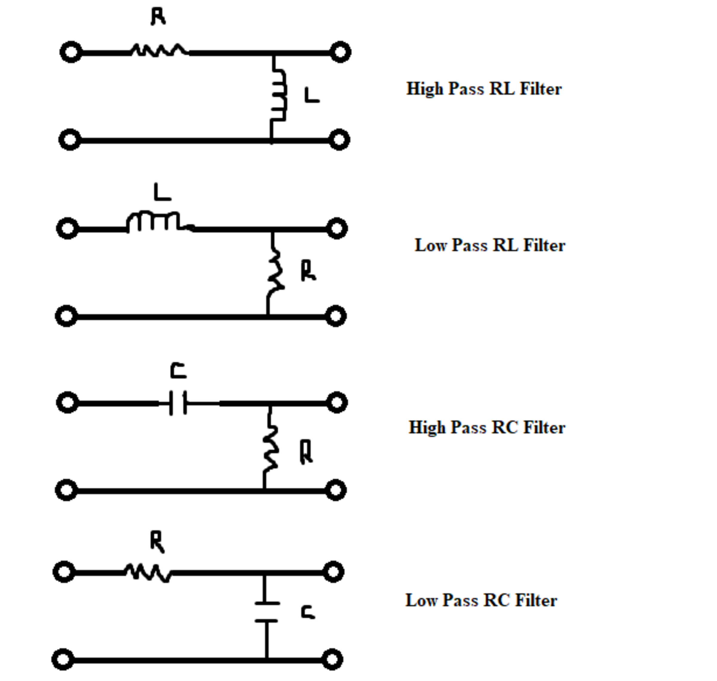
It is important to note that if one can avoid the use of an inductor and can use a capacitor instead then that should be done. This is due to the fact that inductors will be susceptible to magnetic flux going through its loops which can give rise to additional current in the conductor. Since this would cause the circuit to behave in an unexpected manner it should be avoided if possible.

Next let us consider the frequency response of filters, starting with a simple passive first-order low-pass RC filter. The frequency response of a low-pass RC filter is different from a low-pass RL filter which is different again from a low-pass RLC filter. The low-pass RLC filter is of course a second order circuit and this will make the math significantly more difficult. For now we will stick to the first-order circuits. The frequency response graphs of all low-pass filters will be very similar, but the equations will have different variables. This is also true for the high-pass filters. The frequency response graphs will have similar shapes, but the equations will have different variables.

PASSIVE FIRST ORDER LOW-PASS RC FILTER

The low-pass filter will provide voltage at its output terminal but it is dependent on the frequency of the input signal. The low-pass filter will let signals pass at all low frequencies up until a certain frequency called the cutoff frequency where the amplitude of the voltage wave at the output will be less than or equal to the input voltage divided by the square root of two (this is the effective value of the input voltage) . In other words at frequencies above the cutoff frequency the amplitude of the output is significantly diminished and we say that those frequencies have been filtered out since they do not provide a strong enough signal at the output. Since this type of filter lets signals through at low frequencies it is called a low-pass filter. Signals can pass through the filter at low frequencies but they are unable to pass if the frequency is above the cutoff frequency. Let us consider the low-pass RC filter. This circuit acts as a voltage divider splitting the total voltage between the resistor and the capacitor based on the ratio of the impedance of each component to the total impedance. Provided that some input voltage signal is applied across the input terminals then the voltage across the output terminals is given by the following equation.

$v_{o} = v_{i} \frac{X_{c}}{Z}$

At the cutoff frequency the voltage is split evenly between the two components. The magnitude of the capacitive reactance of the circuit is equal to the magnitude of the resistance of the circuit and the magnitude of the voltage vectors for the two components are equal. Since it is a series circuit the magnitude of the current vectors will also be equal. If both the current and voltage have the same magnitude then the magnitude of the power dissipated across each component will also be equal. All of these properties define the cutoff frequency. We can use the magnitude of impedance formula to draw some conclusions about the circuit at the cutoff frequency.

$|X_{c}| = |R|$

$|Z|= \sqrt{|X_{c}|^{2} + |R|^{2}}$

$|Z|= \sqrt{|R|^{2} + |R|^{2}}=\sqrt{|X_{c}|^{2}+ |X_{c}|^2}$

$|Z|= \sqrt{2|R|^{2}}= \sqrt{2|X_{c}|^{2}}$

$|Z|= \sqrt{2}|R|=\sqrt{2}|X_{c}|$

Naturally, this implies that at the cutoff frequency the output voltage is equal to the input voltage divided by the square root of two.

$\frac{|v_{i}|}{\sqrt{2}} = |v_{i}| \frac{|X_{c}|}{|Z|}$

$\frac{1}{\sqrt{2}} = \frac{|X_{c}|}{|Z|}$

$|Z| = \sqrt{2} |X_{c}|$

Now we can find the cutoff frequency from the formula for capacitive reactance. The capacitive reactance is equal to the magnitude of the resistance.

$|X_{c}| =|R|$

$\frac{1}{2 \pi f_{c} C} =R$

$f_{c} =\frac{1}{2 \pi R C}$

If we now would like to plot the output voltage as a function of frequency of the input we simplify the following equation.

$v_{o} = v_{i} \frac{X_{c}}{Z}$

$v_{o} = v_{i} \frac{\frac{1}{2\pi fC} \angle -\frac{\pi }{2}}{R \angle 0 +\frac{1}{2\pi f C} \angle -\frac{\pi}{2}}$

$v_{o} = v_{i} \frac{\frac{1}{2\pi fC} \angle -\frac{\pi}{2}}{\sqrt{R^{2}+ (\frac{1}{2\pi fC})^{2}} \angle - \tan^{-1}(\frac{\frac{1}{2\pi fC}}{R})}$

Since we have this equation in polar form we can separate the equation into two separate functions. We can write this as one function for the magnitude and one function for the phase angle.

$|v_{o}| = |v_{i}| \frac{1} {2\pi fC\sqrt{R^{2}+ (\frac{1}{2\pi fC})^{2}}}$

$|v_{o}| = |v_{i}| \frac{1} {\sqrt{4 \pi^{2} f^{2}C^{2} (R^{2}+ \frac{1}{4\pi^{2} f^{2}C^{2}}})}$

$|v_{o}| = |v_{i}| \frac{1} {\sqrt{4 \pi^{2} f^{2}C^{2}R^{2}+ \frac{4 \pi^{2} f^{2}C^{2}}{4\pi^{2} f^{2}C^{2}}}}$

$|v_{o}| = |v_{i}| \frac{1} {\sqrt{4 \pi^{2} f^{2}C^{2}R^{2}+ 1}}$

$\phi = -\frac{\pi}{2} + \tan^{-1}(\frac{\frac{1}{2\pi fC}}{R})$

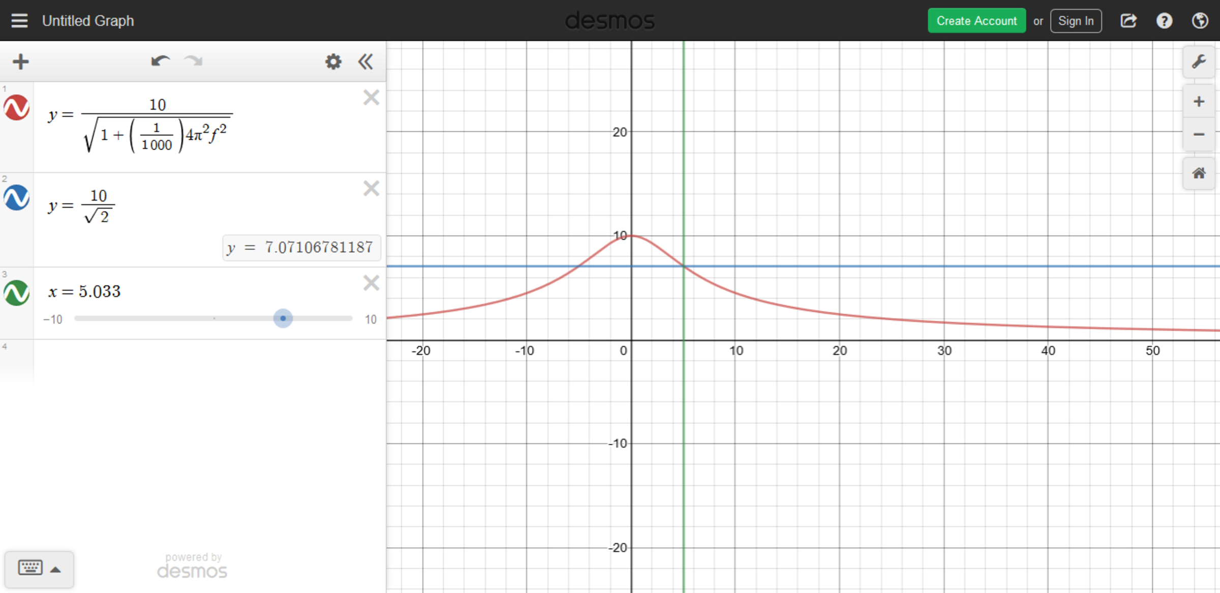
If we set $|v_{i}|=10,R^{2}C^{2}= \frac{1}{1000}$ ($R=31.62$ and $C=\frac{1}{1000}=0.001$) we get a cutoff frequency of about $5 Hz$. This is just of course an example but capacitance values are usually very small in the order of micro Farads. Therefore this graph is a good indication of the frequency response of a low pass filter. The graph of the magnitude of the output voltage is as seen below. I have drawn additional lines to show the point where the cutoff frequency occurs. We only consider the positive frequencies as valid inputs since negative frequencies do not describe anything in reality.

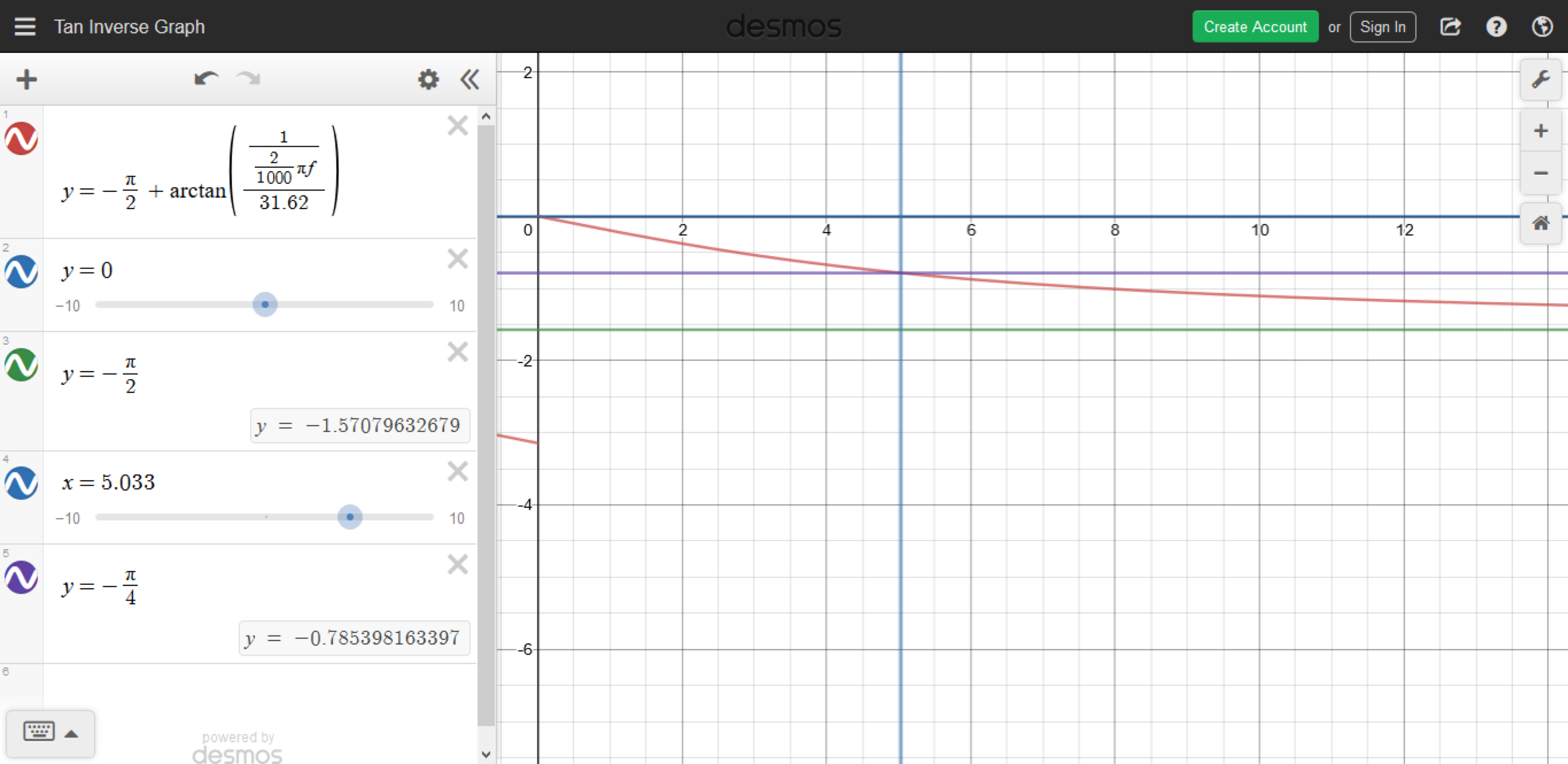
It is important to also understand what the graph of the phase angle looks like. Below we see that at the cutoff frequency of $5 Hz$ the phase angle is $-\frac{\pi}{4}$. Since the minimum phase angle is $-\frac{\pi}{2}$ and the maximum phase angle is $0$ these form the asymptotes for the graph.

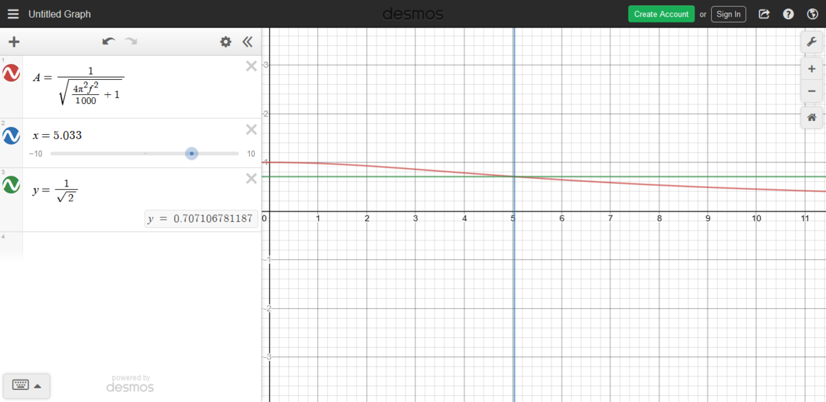
This leads us now to the topic of the gain/attenuation of the voltage of the filter. Gain/attenuation of the voltage is defined as the ratio of output voltage to input voltage. In this case we refer to it as attenuation since the signal strength is being decreased by some factor.

$A_{v}= \frac{v_{o}}{v_{i}}$

$A_{v}= \frac{1}{\sqrt{1+(2\pi f RC)^{2}}} \angle - \frac{\pi}{2}+ \tan ^{-1}(\frac{\frac{1}{2\pi fC}}{R})$

$A_{v} = \frac{1} {\sqrt{4 \pi^{2} f^{2}C^{2}R^{2}+ 1}} \angle -\frac{\pi}{2}+ \tan ^{-1}(\frac{1}{2\pi fCR})$

Of course the angle can be simplified by using algebraic methods. We can convert the equation from polar form to rectangular form. To do this we express the phase angle of $-\frac{\pi}{2}$ as a multiplication by $-j$ and then treat it as any variable. An important identity we will use is that $\frac{1}{j} = -j$.

$A_{v}= \frac{X_{c}}{Z}$

$A_{v}= \frac{\frac{1}{2\pi fC} \angle -\frac{\pi }{2}}{R \angle 0 +\frac{1}{2\pi f C} \angle -\frac{\pi}{2}}$

$A_{v}= \frac{\frac{-j}{2\pi fC}}{R +\frac{-j}{2\pi f C}}$

$A_{v}= \frac{\frac{1}{2\pi fCj}}{R +\frac{1}{2\pi f Cj}}$

$A_{v}= \frac{1}{R2\pi fCj +1}$

Now we can convert back to polar form to separate the equation into two functions. We will split the equation up into one function for the magnitude and one function for the phase angle.

$A_{v} = \frac{1\angle 0} {\sqrt{4 \pi^{2} f^{2}C^{2}R^{2}+ 1} \angle\tan ^{-1}(\frac{2\pi fCR}{1})}$

$A_{v} = \frac{1\angle 0} {\sqrt{4 \pi^{2} f^{2}C^{2}R^{2}+ 1} \angle\tan ^{-1}(2\pi fCR)}$

$A_{v} = \frac{1} {\sqrt{4 \pi^{2} f^{2}C^{2}R^{2}+ 1}}\angle -\tan ^{-1}(2\pi fCR)$

Now we can look at the graphs for gain/attenuation which will look very similar to the graphs for the output voltage. The attenuation is a number between 0 and 1. A phase shift is also applied.

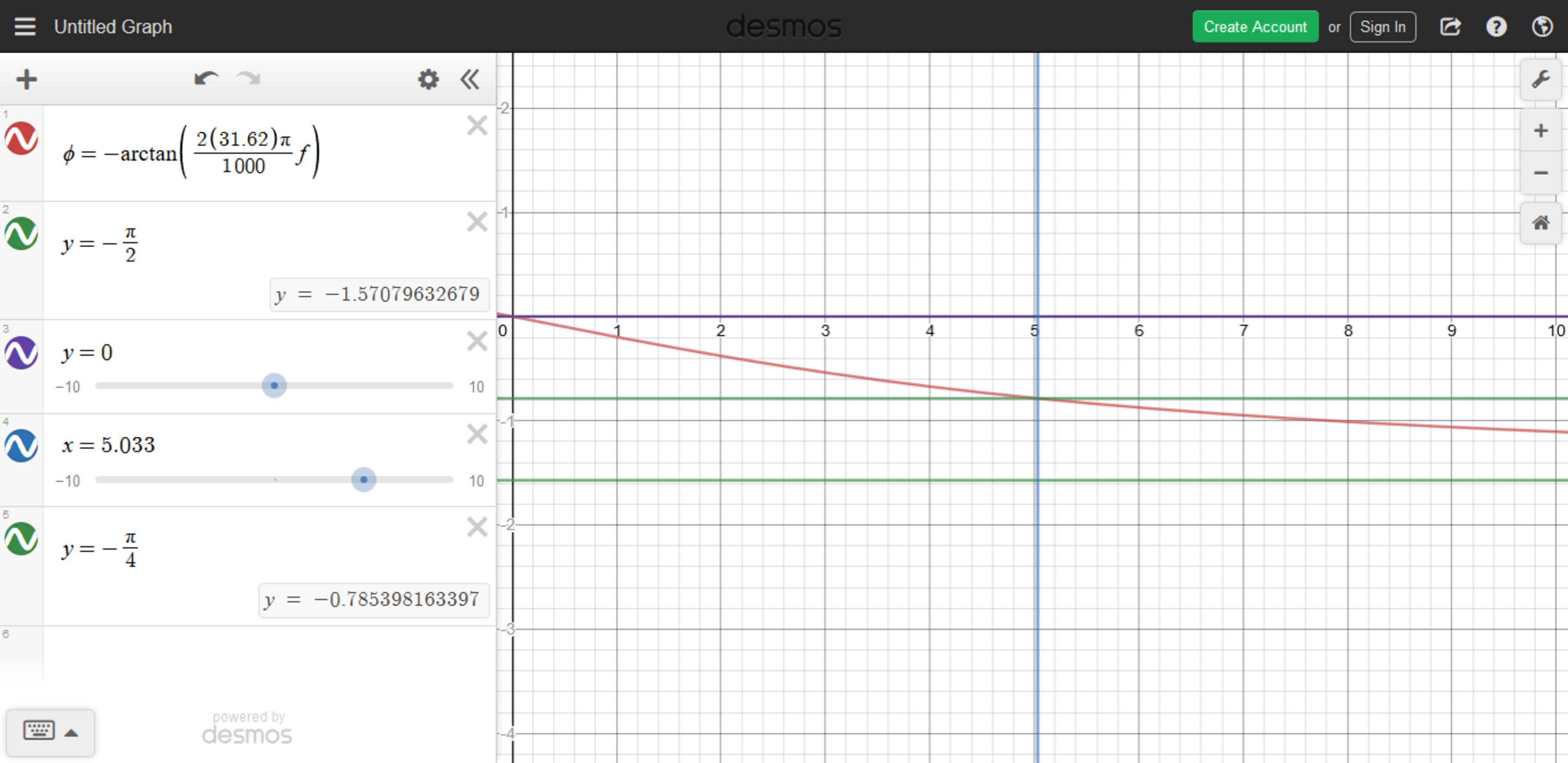
We can of course write the same equation for the attenuation of the voltage of the filter in terms of the ratio between the frequency and the cutoff frequency. We already know how to find the cutoff frequency. Let us work from that.

$f_{c}=\frac{1}{2\pi CR}$

$\frac{1}{f_{c}}=2\pi CR$

$\frac{f}{f_{c}}=2\pi fCR$

We can substitute this into the attenuation equation.

$A_{v} = \frac{1} {\sqrt{(\frac{f}{f_{c}})^{2}+ 1}}\angle -\tan ^{-1}(\frac{f}{f_{c}})$

The next thing we will consider is the power of the circuit. Power is the product of the voltage and the current. At the cutoff frequency the magnitude of the voltage and the current at the output have both been attenuated by a factor of $\frac{1}{\sqrt{2}}$ and since$(\frac{1}{\sqrt{2}})^{2} =\frac{1}{2}$ we can conclude that the magnitude of the output power has been attenuated by a factor of one half. This means that at the cutoff frequency the circuit the magnitude of the power is reduced by half. This is called the half-power point.

$|P_{o}|= |v_{o}||i_{o}|$

$|P_{c}|= |v_{c}||i_{c}|$

$|P_{c}|= \frac{|v_{i}|}{\sqrt{2}}\frac{|i_{i}|}{\sqrt{2}}$

$|P_{c}|= \frac{|v_{i}||i_{i}|}{{2}}$

$|P_{c}|= \frac{|P_{i}|}{{2}}$

Power can be measured in watts but when we are talking about the attenuation of the power it can be measured in decibels. The decibel is a logarithmic unit which can be useful for displaying information on both the large and small scale at the same time. It is therefore important to understand how to graph the attenuation of power on the logarithmic scale. The power at a given node is always in reference to the power at some other node. We will use the magnitude of the input power as the reference and then compare the power at the output at each frequency to that maximum to display the attenuation of power in decibels. The attenuation of power does not have to be expressed in decibels but it is a matter of convenience.

$P_{dB} =10 \log{\frac{|P_{o}|}{|P_{i}|}}$

If the power measured at the output node is equal to double the power measured at the input node then the ratio of $\frac{|P_{0}|}{|P_{i}|}$ is equal to $2$ which corresponds to about $3 dB$.

$P_{dB} =10 \log{2}$

$P_{dB} =10 (0.301...)$

$P_{dB} \approx 3$

If the power measured at the output node is equal to half the power measured at the input then the ratio of $\frac{|P_{o}|}{|P_{i}|}$ is equal to $0.5$ which corresponds to about $-3 dB$.

$P_{dB} =10 \log{0.5}$

$P_{dB} =10 (-0.301...)$

$P_{dB} \approx -3$

Another way to express the power is in terms of the voltage.

$P=VI$

$P=\frac{V^{2}}{R}$

$P=I^{2}R$

Therefore we can write the attenuation of power in decibels in terms of the voltage or current as well. I will show how this is done for voltage.

$P_{dB}=10 \log(\frac{\frac{|v_{o}|^{2}}{R}}{\frac{|v_{i}|^{2}}{R}})$

$P_{dB}=10 \log(\frac{|v_{o}|^{2}}{|v_{i}|^{2}})$

$P_{dB}=10 \log((\frac{|v_{o}|}{|v_{i}|})^{2})$

$P_{dB}=2 \times 10 \log(\frac{|v_{o}|}{|v_{i}|})$

$P_{dB}=20 \log(\frac{|v_{o}|}{|v_{i}|})$

If the voltage measured at the output is equal to double the power measured at moment one then the ratio of $\frac{|v_{o}|}{|v_{i}|}$ is equal to $2$ which corresponds to about $6 dB$.

$P_{dB}=20 \log(2)$

$P_{dB} \approx 6 dB$

If the voltage measured at the output is equal to half the power measured at moment one then the ratio of $\frac{|v_{o}|}{|v_{i}|}$ is equal to $0.5$ which corresponds to about $-6 dB$.

$P_{dB}=20 \log(0.5)$

$P_{dB} \approx -6 dB$

Since we already found the expression for the attenuation of the voltage we can substitute that into the equation for attenuation of power.

$P_{dB}=20 \log(\frac{|v_{o}|}{|v_{i}|})$

$P_{dB}=20 \log(|A_{v}|)$

$P_{dB}= 20 \log(\frac{1} {\sqrt{(\frac{f}{f_{c}})^{2}+ 1}})$

Regular graphing software won't work this time since we want to plot this curve on a logarithmic scale. One method is to take some sample points and the use excel to plot the curve. Excel allows you to set the axis scale to a logarithmic scale. On this scale we can approximate the curve as a piecewise function composed of two linear functions. This type of approximation is called a bode plot. I have not drawn the bode plot but it is easy to see how this curve could be approximated by a piecewise function composed of two straight lines. I will describe the piecewise function below.

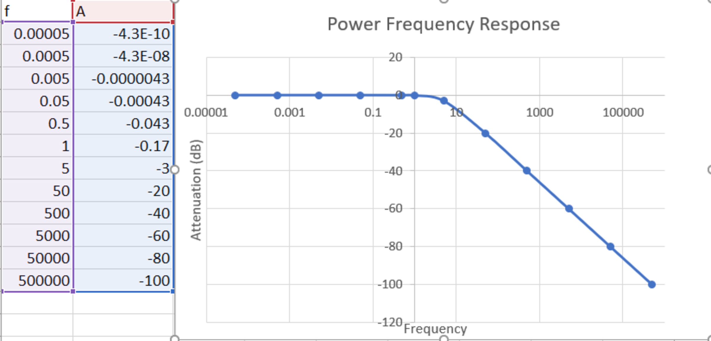
Up until the cutoff frequency we can approximate the attenuation curve in decibels as the line $y=0$. After that we can approximate the curve as a linear function with a slope of $-20dB$ per decade (power of 10) and a horizontal shift of $f_c$. Of course this results in a discontinuity at $f= f_{c}$.

When $f<f_{c}$, then $(\frac{f}{f_{c}})^{2} <1$. Therefore the attenuation formula simplifies if we ignore the $\frac{f}{f_{c}}$ term in the attenuation of power formula.

$P_{dB} \approx 20 \log(\frac{1} {\sqrt{1}}), f<f_{c}$

$P_{dB} \approx 20 \log(1), f<f_{c}$

$P_{dB} \approx 20 (0), f<f_{c}$

$P_{dB} \approx 0, f<f_{c}$

When $f>f_{c}$, then $(\frac{f}{f_{c}})^{2} >1$. Therefore the attenuation formula simplifies if we ignore the $+ 1$ term in the attenuation of power formula.

$P_{dB} \approx 20\log(\frac{1}{\sqrt{(\frac{f}{f_{c}}})^{2}}) , f> f_{c}$

$P_{dB} \approx 20\log(\frac{f_{c}}{f}) , f> f_{c}$

$P_{dB} \approx 20\log(f_{c}) -20\log(f) , f>f_{c}$

The first term $20\log(f_{c})$ is the vertical shift of the linear function and the $-20$ that scales the $\log(f)$ term is the slope on the logarithmic scale. The slope is $-20dB$ per decade (power of ten).

In summary the attenuation of the power on the logarithmic scale can be expressed as a piecewise function called a bode plot. We use two separate linear functions to approximate this curve.

$P_{dB} \approx 0, f<f_{c}$

$P_{dB} \approx 20\log(f_{c}) -20\log(f) , f>f_{c}$

We can also express voltage attenuation or current attenuation in decibels. Any ratio that represents the gain/attenuation can be expressed in decibels. We can do bode plots for both the magnitude and the phase angle. For the bode plot of the phase angles we have to use a piecewise function that is made up of three linear functions. This results in discontinuities at$f= \frac{f_c}{10}$ and $f= 10f_{c}$. The important thing to remember is that bode plots are always done on a logarithmic scale.

The final thing to discuss about the filter is its bandwidth. In analog circuits the bandwidth is defined as the width of the pass-band. In the case of the low pass filter the passband is $0Hz-f_{c}Hz$ so the bandwidth is $f_{c}-0$ or just $f_{c}$.

PASSIVE FIRST ORDER HIGH-PASS RC FILTER

Since I have done such a detailed analysis of the first order low-pass filter I will now try to go through the first order high-pass filter a little more quickly since most of the concepts are similar to those of the low-pass filter. To find the output voltage we can use the voltage divider equation except this time the output voltage will be the voltage across the resistor.

$v_{o} = v_{i} \frac{R}{Z}$

Therefore we can express the attenuation of voltage with the following equation.

$A_{v}= \frac{v_{o}}{v_{i}}$

$A_{v}= \frac{R}{Z}$

$A_{v}= \frac{R \angle 0}{R \angle 0 +\frac{1}{2\pi f C} \angle -\frac{\pi}{2}}$

$A_{v}= \frac{R}{R +\frac{-j}{2\pi f C}}$

$A_{v}= \frac{R}{R +\frac{1}{2\pi f Cj}}$

$A_{v} = \frac{R\angle 0} {\sqrt{R^{2}+ (\frac{1}{2\pi fC})^{2}} \angle-\tan ^{-1}(\frac{1}{2\pi fCR})}$

$A_{v} = \frac{1 \angle0} {\frac{1}{R}\sqrt{R^{2}+ \frac{1}{2^{2}\pi^{2} f^{2}C^{2}}} \angle-\tan ^{-1}(\frac{1}{2\pi fCR})}$

$A_{v} = \frac{1 \angle0} {\sqrt{(\frac{1}{R})^{2}(R^{2}+ \frac{1}{2^{2}\pi^{2} f^{2}C^{2}})} \angle -\tan ^{-1}(\frac{1}{2\pi fCR})}$

$A_{v} = \frac{1 \angle0} {\sqrt{1+ \frac{1}{2^{2}\pi^{2} f^{2}C^{2}R^{2}}} \angle -\tan ^{-1}(\frac{1}{2\pi fCR})}$

$A_{v} = \frac{1} {\sqrt{1+ \frac{1}{2^{2}\pi^{2} f^{2}C^{2}R^{2}}}}\angle \tan ^{-1}(\frac{1}{2\pi fCR})$

$A_{v} = \frac{1} {\sqrt{1+ (\frac{f_{c}}{f})^{2}}}\angle \tan ^{-1}(\frac{f_{c}}{f})$

Now we can graph the magnitude and phase angle as two separate functions. I have also made sure to display the borders that define the curve and the cutoff point for each graph. I have done this using the cutoff frequency from the previous example with the low pass RC filter. The cutoff frequency is about $5HZ$.

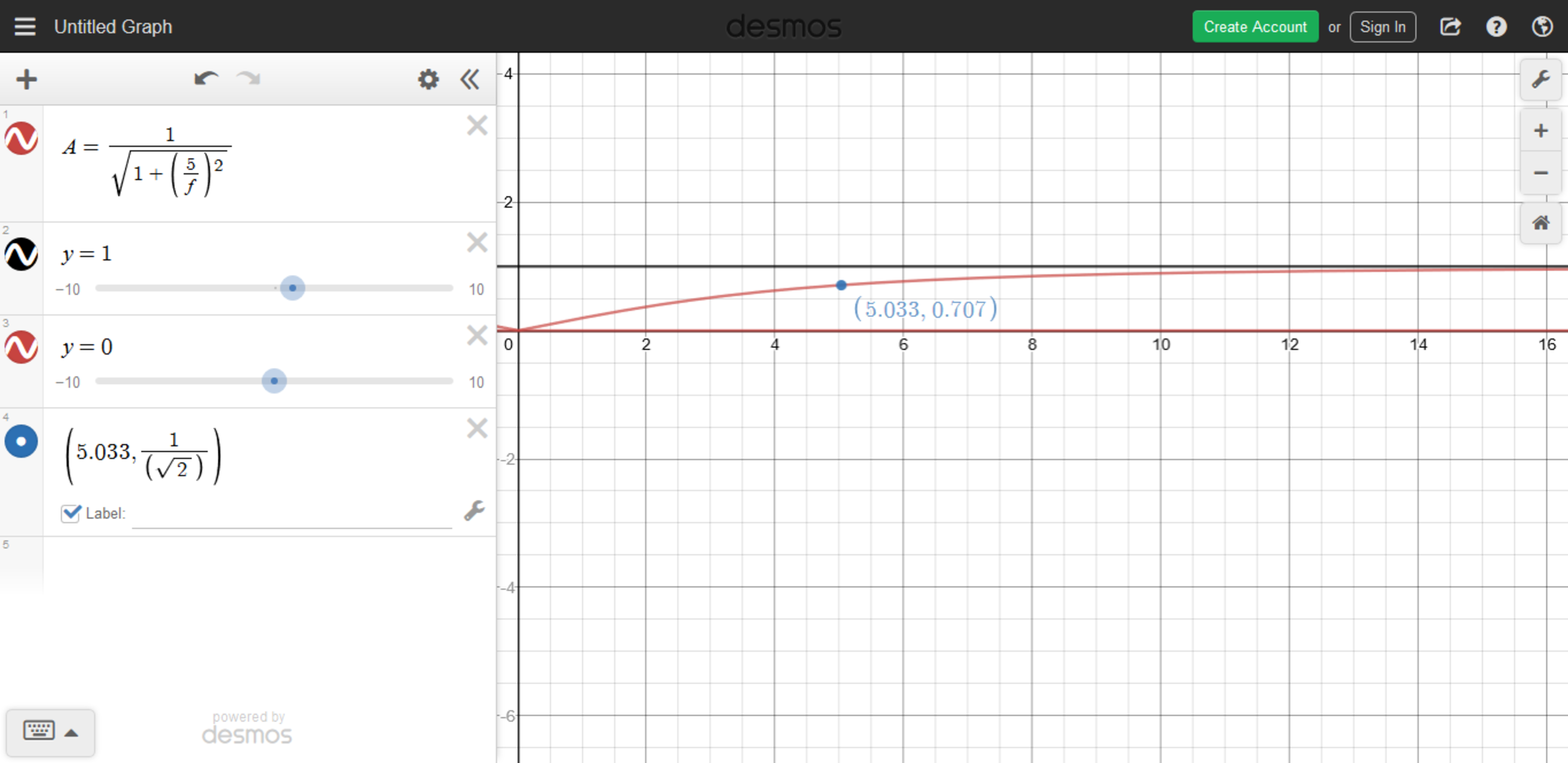
We can plot this on the logarithmic scale as well. Note that I have not yet converted this to decibels. It is just a unit-less ratio but the frequency axis has been changed to the logarithmic scale.

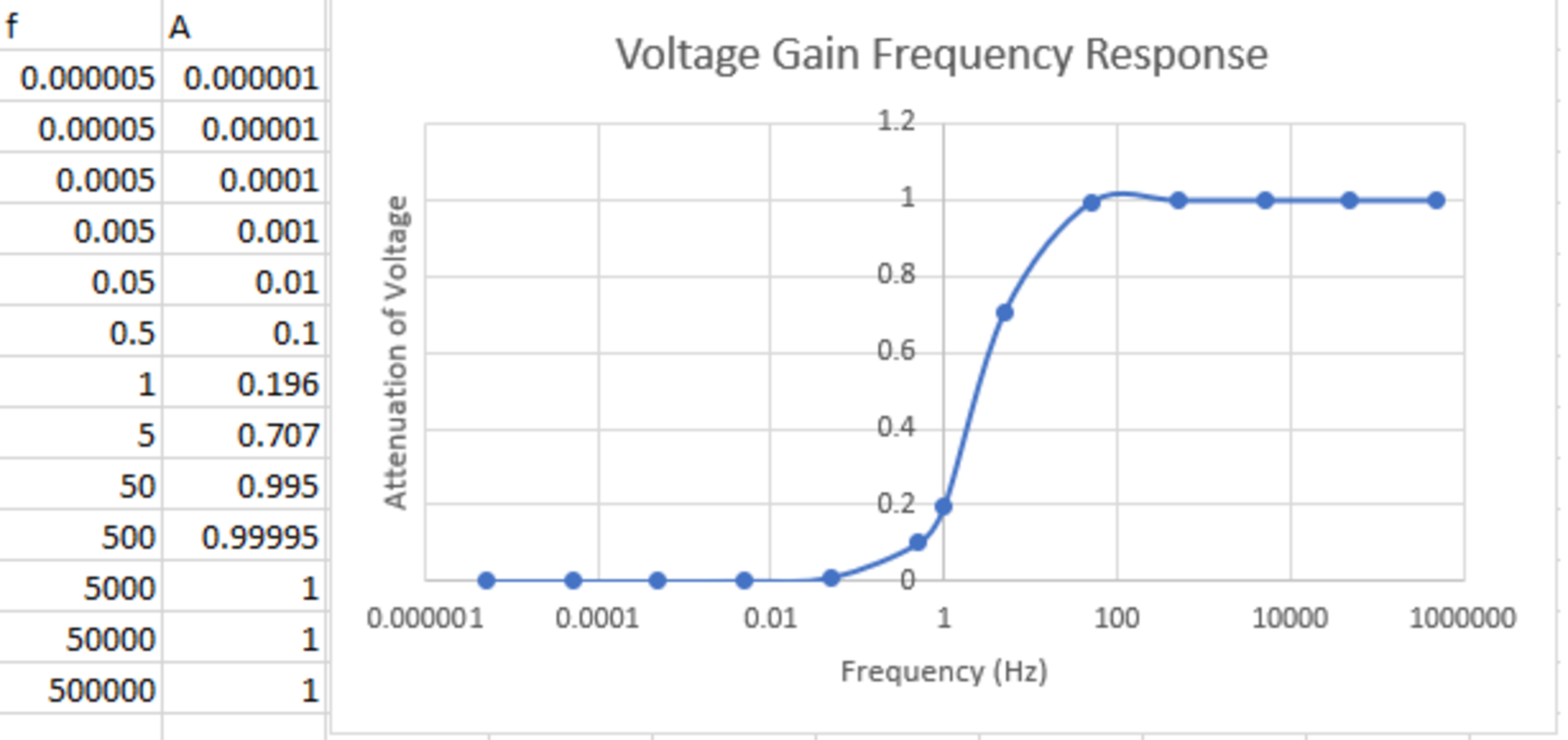
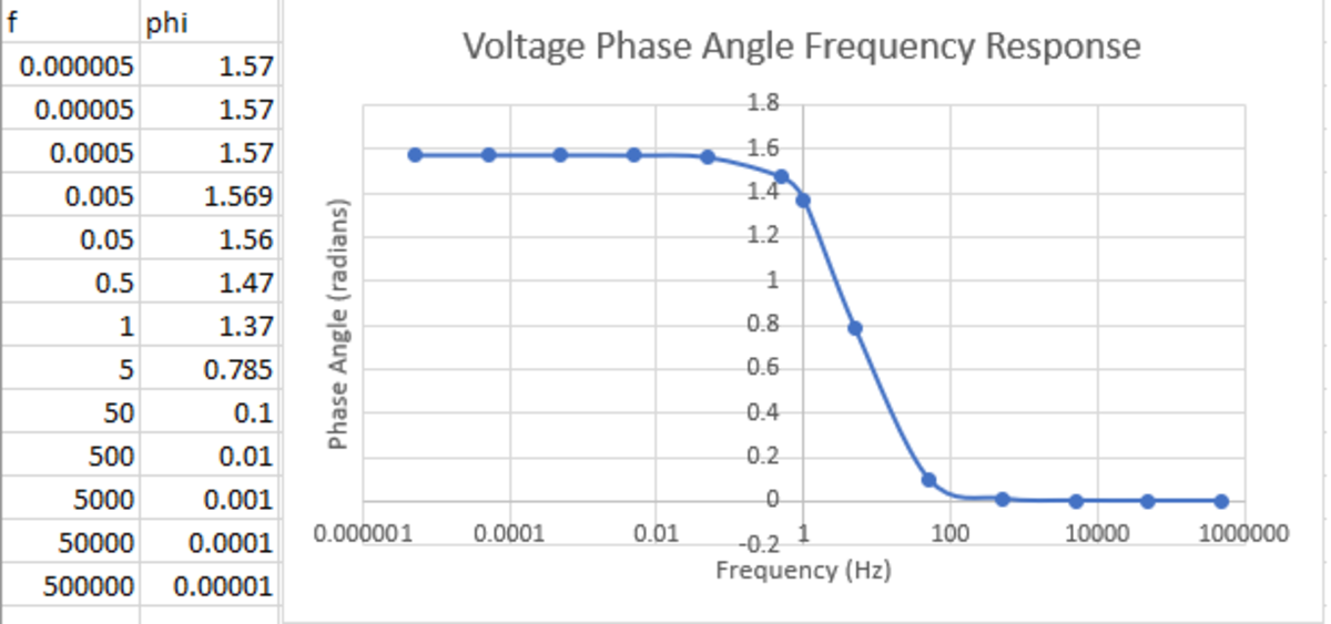
We can also plot the voltage magnitude attenuation on the logarithmic scale by using units of decibels. This is shown below. Note the slope for voltage attenuation is $-10dB$ per decade.

$A_{v}= 10 log (A_{v}) (dB)$

$A_{v}= 10 log (\frac{1}{\sqrt{1+(\frac{f_{c}}{f})^2}}) (dB)$

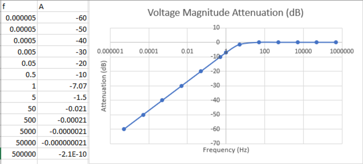
It is easy to see how these curves can be approximated by using the bode plot so I will not show that again for this filter.