Plotting Electric Dipole Field Lines

The net electric field vector can be calculated at any point in the vicinity of an electric dipole. Each point in space can therefore be associated with a directional unit vector indicating the field's direction. We can follow these vectors, taking tiny steps along the field lines to get from one charge to the other, plotting the field lines as we go. The high-level process is:

1) Set up many departure points around the first charge, arrayed in a circle. Start points are initialized a small distance away from charge 1, at various angles. Each start point is associated with a distinct field line which starts near charge 1 and ends near charge 2.

2) To move from one point on the field line to another, first calculate the net electric field vector at the point. Then create a unit-direction vector based on the E-field. Then move a tiny distance "epsilon" in the direction of the unit vector to get to the next point on the field line. Continue along a particular field line until arriving at charge 2.

3) Upon arriving at charge 2, end the present field line, initialize a new departure point around charge 1, and trace out the next field line.

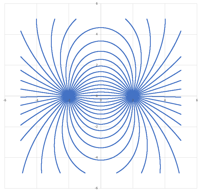
Example Plot:

Interestingly, we can see that the lines are closer where the field should be stronger. This feature "emerges" from the plotting process, without having to be explicitly coded.

Code:

import math

# Constants

k = 3.7

q1 = 1.0
q2 = -1.0

x1 = -2.0
y1 = 0.0

x2 = 2.0
y2 = 0.0

delta = 10.0**(-3.0)

# Departure angle resolution

dtheta = 2.0 * math.pi / 40.0

theta = dtheta / 7.0

# Starting radius

rst = 0.01

# Count decouples sim resolution from print resolution

count = 0

while theta <= 2.0 * math.pi:    # Departure points all around charge 1

    x = x1 + rst * math.cos(theta)
    y = y1 + rst * math.sin(theta)

    d2 = 999999999.0

    while d2 > rst:             # Follow field lines until arriving at charge 2

        dx1 = x - x1
        dy1 = y - y1

        dx2 = x - x2
        dy2 = y - y2

        d1 = math.hypot(dx1,dy1)
        d2 = math.hypot(dx2,dy2)

        ux1 = dx1 / d1
        uy1 = dy1 / d1

        ux2 = dx2 / d2
        uy2 = dy2 / d2

        E1mag = k*q1 / (d1**2.0)
        E2mag = k*q2 / (d2**2.0)

        Ex1 = E1mag * ux1
        Ey1 = E1mag * uy1

        Ex2 = E2mag * ux2
        Ey2 = E2mag * uy2

        Ex = Ex1 + Ex2
        Ey = Ey1 + Ey2

        Emag = math.hypot(Ex,Ey)

        uEx = Ex / Emag
        uEy = Ey / Emag

        x = x + delta * uEx
        y = y + delta * uEy

        if (math.fabs(x) < 5.0) and (math.fabs(y) < 5.0) and (count % 10 == 0):

            print x,y

        count = count + 1


    theta = theta + dtheta