Already with a single qubit you can perform complicated operations, because you can make arbitrary superpositions of the two basis states. However, it only becomes interesting when you have a memory register with many qubits available. Now, operations such as the CNOT gate, linking multiple qubits, are also possible. In this way, qubits can be entangled with each other, so that their states are correlated with each other and can no longer be considered separately. This entanglement provides a new way to store information and perform calculations, which is not possible with a classical computer.
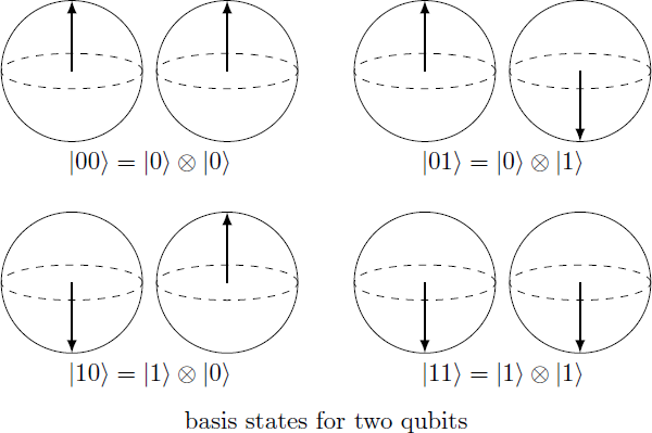
Two qubit states
We consider a system of two qubits. If both qubits are measured, there can be in one of four possible states. These basis states ∣00⟩, ∣01⟩, ∣10⟩ and ∣11⟩ result mathematically as tensor product of the single basis states:
∣00⟩=∣0⟩⊗∣0⟩∣01⟩=∣0⟩⊗∣1⟩∣10⟩=∣1⟩⊗∣0⟩∣11⟩=∣1⟩⊗∣1⟩≡(10)⊗(10)=⎝⎜⎜⎛1000⎠⎟⎟⎞≡(10)⊗(01)=⎝⎜⎜⎛0100⎠⎟⎟⎞≡(01)⊗(10)=⎝⎜⎜⎛0010⎠⎟⎟⎞≡(01)⊗(01)=⎝⎜⎜⎛0001⎠⎟⎟⎞
The general state ∣ψ⟩ of the quantum system can be represented as a superposition of base states and thus corresponds to a four-dimensional vector:
∣ψ⟩=α∣00⟩+β∣01⟩+γ∣10⟩+δ∣11⟩≡⎝⎜⎜⎛αβγδ⎠⎟⎟⎞∈C4
If this state is normalized (i.e. ∣α∣2+∣β∣2+∣γ∣2+∣δ∣2=1), then the absolute squares ∣α∣2,∣β∣2,∣γ∣2 and ∣δ∣2 correspond to the probabilities to measure the respective state.
∣ψ⟩≡⎝⎜⎜⎛αβγδ⎠⎟⎟⎞⟶measurement∣ψ′⟩=⎩⎪⎪⎪⎨⎪⎪⎪⎧∣00⟩∣01⟩∣10⟩∣11⟩with probability ∣α∣2with probability ∣β∣2with probability ∣γ∣2with probability ∣δ∣2
Separable and entangled states
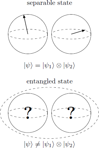
The state ∣ψ⟩ of a two-qubit system is called separable if the two qubits do not depend on each other. In this case, the state can be written as a tensor product of individual states:
∣ψ⟩=∣ψ1⟩⊗∣ψ2⟩=(α1∣0⟩+β1∣1⟩)⊗(α2∣0⟩+β2∣1⟩)≡(α1β1)⊗(α2β2)=⎝⎜⎜⎛α1α2α1β2β1α2β1β2⎠⎟⎟⎞
It is therefore possible to specify separately the states ∣ψ1⟩ and ∣ψ2⟩ of the first and second qubit. In particular, the basis states ∣00⟩,∣01⟩,∣10⟩ and ∣11⟩ are separable.
In the general case, however, the quantum state can not be separated because the qubits depend on each other. In this case there is an entangled state or an entanglement. This is indicated by the fact that the measurements of different qubits provide random outcomes, but the results are correlated with each other. A special case are maximum entangled states, in which the measurement result of the first qubit completely defines the state of the second qubit.
Bell state
Is the state
∣ψ⟩=21(∣00⟩+∣11⟩)
separable or entangled?
When measuring both qubits, the states ∣00⟩ and ∣11⟩ result with equal probability, so that at the end both qubits must be in the same basis state. Whether the one qubit assumes the state ∣0⟩ or ∣1⟩ is not set in advance and depends on the other qubit. Thus, the two qubits can no longer be considered separately and there is no decomposition in the form ∣ψ⟩=∣ψ1⟩⊗∣ψ2⟩. Futhermore, the state ∣ψ⟩ is maximum entangled, since a measurement of a single qubit determines the state of the other qubit.
Two-qubit gates
The state of the two-qubit system can also be manipulated with quantum gates, which are now represented by unitary 4×4 matrices. The application of a gate U corresponds to the matrix mutiplication with the four-dimensional state vector:
UU∣ψ⟩≡⎝⎜⎜⎛u11u21u31u41u12u22u32u42u13u23u33u43u14u24u34u44⎠⎟⎟⎞∈C4×4,∣ψ⟩≡⎝⎜⎜⎛αβγδ⎠⎟⎟⎞∈C4≡⎝⎜⎜⎛u11u21u31u41u12u22u32u42u13u23u33u43u14u24u34u44⎠⎟⎟⎞⋅⎝⎜⎜⎛αβγδ⎠⎟⎟⎞=⎝⎜⎜⎛αu11+βu12+γu13+δu14αu21+βu22+γu23+δu24αu31+βu32+γu33+δu34αu41+βu42+γu43+δu44⎠⎟⎟⎞
Single-qubit gates
The single-qubit gates that we have come to know so far can also be transferred to the two-qubit system. Let U be such a one-qubit gate then one can now define two-qubit operators U1=U⊗I and U2=I⊗U, each corresponding to the application of U to the first or second qubit. The new operators are defined by their effect on the base states
U1∣ij⟩U2∣ij⟩=(U⊗I)∣ij⟩=(U∣i⟩)⊗∣j⟩=(I⊗U)∣ij⟩=∣i⟩⊗(U∣j⟩)
where i,j∈{0,1}. Using this rule, the matrix representation of this operators can also be derived:
UU1U2=(acbd)∈C2×2=U⊗I≡⎝⎜⎜⎛a0c00a0cb0d00b0d⎠⎟⎟⎞=I⊗U≡⎝⎜⎜⎛ac00bd0000ac00bd⎠⎟⎟⎞
Controlled NOT (CNOT)
Besides single-qubit operations, we also need additional operations that can link the two qubits together and create an entanglement. An example of such an operation is the Controlled-NOT gate (CNOT), which can be described by the following matrix:
CNOT=⎝⎜⎜⎛1000010000010010⎠⎟⎟⎞∣ψ⟩∣00⟩∣01⟩∣10⟩∣11⟩CNOT∣ψ⟩∣00⟩∣01⟩∣11⟩∣10⟩
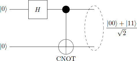
The first qubit is called control bit and the second bit target bit. In the diagram, the target bit is marked with a cross and is connected with a line to the control bit. The CNOT gate applies a NOT operation (X-gate) to the target bit if and only if the control bit is in the state ∣1⟩.
Using the CNOT gate and the Hadamard gate, the Bell state can be generated from an initial state ∣00⟩:
CNOT⋅(H⊗I)⋅∣00⟩=CNOT⋅21(∣00⟩+∣10⟩)=21(∣00⟩+∣11⟩)
This discussion board is a place to discuss our Daily Challenges and the math and science
related to those challenges. Explanations are more than just a solution — they should
explain the steps and thinking strategies that you used to obtain the solution. Comments
should further the discussion of math and science.
When posting on Brilliant:
Use the emojis to react to an explanation, whether you're congratulating a job well done , or just really confused .
Ask specific questions about the challenge or the steps in somebody's explanation. Well-posed questions can add a lot to the discussion, but posting "I don't understand!" doesn't help anyone.
Try to contribute something new to the discussion, whether it is an extension, generalization or other idea related to the challenge.
Stay on topic — we're all here to learn more about math and science, not to hear about your favorite get-rich-quick scheme or current world events.
Markdown
Appears as
*italics* or _italics_
italics
**bold** or __bold__
bold
- bulleted
- list
bulleted
list
1. numbered
2. list
numbered
list
Note: you must add a full line of space before and after lists for them to show up correctly
    # I indented these lines
    # 4 spaces, and now they show
    # up as a code block.

    print "hello world"
# I indented these lines
# 4 spaces, and now they show
# up as a code block.

print "hello world"
Math
Appears as
Remember to wrap math in \( ... \) or \[ ... \] to ensure proper formatting.
2 \times 3
2×3
2^{34}
234
a_{i-1}
ai−1
\frac{2}{3}
32
\sqrt{2}
2
\sum_{i=1}^3
∑i=13
\sin \theta
sinθ
\boxed{123}
123
Comments
Thanks for the notes! I appreciate the pictures especially, clearly you put quite some work into this. Actually, I was looking into this stuff before (inspired by codeforces Q# competition), and I just wanted to share this article too for anyone looking into this stuff https://www.scottaaronson.com/democritus/lec9.html, because it offers a pretty different way of looking at it that I found complimentary and interesting
Thanks for the encouragement. I always try to summarize the essence of the topic in these notes without going too much into detail. Of course, these notes are not a substitute for a complete lecture or textbook. But it's hard to find a textbook that will allow beginners getting in quantum computing and to write some own programs. That's why I find this article by Scott Aaronson particularly interesting and will take a closer look at it again. Thanks!
 The general state of the quantum system can be represented as a superposition of base states and thus corresponds to a four-dimensional vector:
If this state is normalized (i.e. ), then the absolute squares and correspond to the probabilities to measure the respective state.
The general state of the quantum system can be represented as a superposition of base states and thus corresponds to a four-dimensional vector:
If this state is normalized (i.e. ), then the absolute squares and correspond to the probabilities to measure the respective state.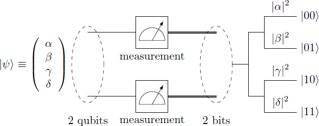
 The state of a two-qubit system is called separable if the two qubits do not depend on each other. In this case, the state can be written as a tensor product of individual states:
It is therefore possible to specify separately the states and of the first and second qubit. In particular, the basis states and are separable.
The state of a two-qubit system is called separable if the two qubits do not depend on each other. In this case, the state can be written as a tensor product of individual states:
It is therefore possible to specify separately the states and of the first and second qubit. In particular, the basis states and are separable.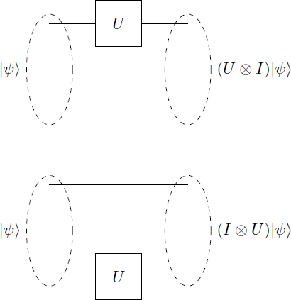
The first qubit is called control bit and the second bit target bit. In the diagram, the target bit is marked with a cross and is connected with a line to the control bit. The CNOT gate applies a NOT operation (X-gate) to the target bit if and only if the control bit is in the state .
Easy Math Editor
This discussion board is a place to discuss our Daily Challenges and the math and science related to those challenges. Explanations are more than just a solution — they should explain the steps and thinking strategies that you used to obtain the solution. Comments should further the discussion of math and science.
When posting on Brilliant:
*italics*or_italics_**bold**or__bold__paragraph 1
paragraph 2
[example link](https://brilliant.org)> This is a quote# I indented these lines # 4 spaces, and now they show # up as a code block. print "hello world"\(...\)or\[...\]to ensure proper formatting.2 \times 32^{34}a_{i-1}\frac{2}{3}\sqrt{2}\sum_{i=1}^3\sin \theta\boxed{123}Comments
Thanks for the notes! I appreciate the pictures especially, clearly you put quite some work into this. Actually, I was looking into this stuff before (inspired by codeforces Q# competition), and I just wanted to share this article too for anyone looking into this stuff https://www.scottaaronson.com/democritus/lec9.html, because it offers a pretty different way of looking at it that I found complimentary and interesting
Log in to reply
Thanks for the encouragement. I always try to summarize the essence of the topic in these notes without going too much into detail. Of course, these notes are not a substitute for a complete lecture or textbook. But it's hard to find a textbook that will allow beginners getting in quantum computing and to write some own programs. That's why I find this article by Scott Aaronson particularly interesting and will take a closer look at it again. Thanks!