Stochastic processes sampler pack (I)

Here we will solve a few classic problems in probability using some exotic methods from non-equilibrium statistical mechanics. Though each of these problems can be addressed using more elementary methods, the tools and tricks we'll explore here are powerful, and can be used to great effect in solving more difficult kinds of questions in physics and probability.

What sets stochastic processes apart from the usual questions in probability is the central role of fluctuations. In stochastic settings, it is not enough to reason about the most likely outcome, as it is not necessarily representative of typical states of the system.

For instance, if we're interested in building a temperature control system for a trip to Mars, it isn't enough to know that the average temperature remains 70 deg F, as this could mean anything from an enjoyable, constant 70 deg F to a ship that switches once a day between 0 and 140 deg F, killing all of its passengers.

For stochastic problems, we'd like to know about all the states of the system and thus require the entire probability distribution.

The first problem that we'll talk about is known, in some circles, as Ehrenfest's urn. In this problem, there are two urns, one on the left ($\mathbf{L}$), and one on the right ($\mathbf{R}$), each of which can hold a total of $N_\text{T}$ balls. At each time step, there is some chance per ball of moving from the left urn to the right urn, and some chance of doing the reverse. Part of the inspiration for this model is the second law of thermodynamics which states roughly that any closed dynamical system will, in the long run, tend to states of highest disorder. If a system is currently in a highly ordered state, it should feel a pressure toward disorder upon rearrangements.

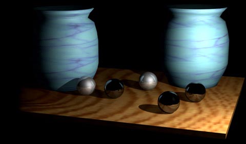
For example, consider a container of liquid after a partition is lifted between pure and dye-containing water:

Here, despite the lack of any identifiable driving force, the ordered (locally concentrated) dye molecules feel an overwhelming pressure to diffuse. An entropic force of sorts drives the system.

The balls in the urn are subject to the same considerations and can therefore bring out the entropic effect, as well as the dynamics of the system as it converges to "thermodynamic" equilbrium. The balls can be replaced with dye, heat, or genes, the effect still holds.

One question we can ask about the urns is what distribution the balls will have, on average, between the two urns. Some harder questions of interest are what dynamics the distribution will have on its way to steady state, and what statistics the steady state distribution of balls will exhibit.

Along the way we'll sketch some powerful results that allow us to make statements about uniqueness.

$\large{\textrm{Urn problem}}$

In the urn problem, we start out with $N_\textrm{L}(0)$ balls in the left urn, and $N_\textrm{R}(0)$ in the right. Each ball in the left urn has a chance $\alpha$ per unit time of moving to the right. Likewise, each ball in the right urn has a chance $\beta$ of moving to the left.

After one time step, the number of balls in the left and right urns has changed to

\begin{alignat}{3} N_\text{L}(\Delta t) \quad & = N_\text{L}(0)\left(1-\alpha\right)\Delta t &&+\quad N_\text{R}(0)\beta \Delta t \\ N_\text{R}(\Delta t) \quad & = N_\text{L}(0)\alpha \Delta t &&+\quad N_\text{R}(0)\left(1-\beta\right)\Delta t \end{alignat}

This can be rewritten in matrix form:

$\overbrace{\begin{pmatrix}N_\text{L}(\Delta t) \\ N_\text{R}(\Delta t)\end{pmatrix}}^{\displaystyle \lvert N_t \rangle} = \overbrace{\begin{pmatrix}1-\alpha \Delta t & \beta \Delta t \\ \alpha \Delta t & 1-\beta\Delta t\end{pmatrix}}^{\displaystyle \mathbb{I} + \mathcal{M}\Delta t}\overbrace{\begin{pmatrix}N_\text{L}(0) \\ N_\text{R}(0)\end{pmatrix}}^{\displaystyle \lvert N_0 \rangle}$

For ease of notation, we write the state of the urns at time $t$ as the vector $\displaystyle\lvert N_t\rangle$. We see that the matrix is the sum of $\mathbb{I} = \begin{pmatrix}1&0\\0&1\end{pmatrix}$ and $\mathcal{M} = \begin{pmatrix}-\alpha & \beta \\ \alpha & -\beta\end{pmatrix}$

Evidently, to move the system through time we multiply the state of the urn by the matrix $\mathbb{I} + \mathcal{M}\Delta t$.

Here, we have a choice to make. We can proceed in continous time (the limit $\Delta t \rightarrow dt$), or in discrete time steps where $\Delta t$ is finite. First, let's look at the continuous time case.

$\large\textrm{Continuous time}$

For simplicity, let us consider the case where $\alpha = \beta = \mu$.

Moving to the continous limit, we have $\Delta t = dt$.

First, we find $\displaystyle \frac{d\lvert N_t\rangle}{dt}$:

$\begin{aligned} \left(\mathbb{I} + \mathcal{M}dt \right) \lvert N_0 \rangle &= \lvert N_{dt} \rangle \\ \mathcal{M}dt\lvert N_{dt}\rangle &= \lvert N_{dt} \rangle - \lvert N_{0} \rangle \\ \mathcal{M}\lvert N_{dt}\rangle &= \frac{\lvert N_{dt} \rangle - \lvert N_{0} \rangle}{dt} \end{aligned}$

and in the limit $dt\rightarrow 0$ we have $\displaystyle\frac{d\lvert N_t\rangle}{dt} = \mathcal{M}\mathcal \lvert N_t\rangle$, which has the solution $\lvert N_t \rangle = e^{\mathcal{M}t}\lvert N_0\rangle$.

Let's unpack the exponential term.

If we write $\gamma = \begin{pmatrix}0 & 1\\ 1 & 0\end{pmatrix}$, we see that $\mathcal{M} = -\mathbb{I} + \gamma$ and so we write

$\begin{aligned} \displaystyle e^{\mathcal{M}t} &= e^{-\mu\mathbb{I}t}e^{\mu\gamma t} \\ &= e^{-\mu\mathbb{I}t}\left(\sum\limits_i \mu^n t^n\frac{\gamma^n}{n!} \right) \\ &= e^{-\mu\mathbb{I}t}\left(\mathbb{I} + \gamma \mu t + \frac{\mu^2 t^2}{2}\gamma^2 + \frac{\mu^3 t^3}{3}\gamma^3 + \ldots\right) \end{aligned}$

This expansion might not seem to help our cause, however, we point out that $\gamma^2 = \begin{pmatrix}0&1\\1&0\end{pmatrix}\begin{pmatrix}0&1\\1&0\end{pmatrix} = \begin{pmatrix}1&0\\0&1\end{pmatrix} = \mathbb{I}$

as do all even powers of $\gamma$. With that identity, we have

$\begin{aligned} e^{-\mu\gamma t} &= \mathbb{I} + \mu t \gamma + \frac{\mu^2 t^2}{2}\mathbb{I} + \frac{\mu^3 t^3}{3}\gamma + \ldots \\ &= \left(\mathbb{I} + \frac{\mu^2 t^2}{2}\mathbb{I} + \ldots\right) + \left( \mu t \gamma + \frac{\mu^3 t^3}{3}\gamma + \ldots\right) \\ &= \cosh\left( \mu t\right)\mathbb{I} + \sinh \left(\mu t\right)\gamma \\ &= \frac12\left(e^{\mu t}+e^{-\mu t}\right)\mathbb{I} + \frac12\left(e^{\mu t}-e^{-\mu t}\right)\mathbb{\gamma} \end{aligned}$

Now,

$\begin{aligned} e^{\mu\mathcal{M}t} &= e^{-\mu t}\mathbb{I}\left[\frac12\left(e^{\mu t}+e^{-\mu t}\right)\mathbb{I} + \frac12\left(e^{\mu t}-e^{-\mu t}\right)\mathbb{\gamma}\right] \\ &= \frac12\left(1+e^{-2\mu t}\right)\mathbb{I} + \frac12\left(1-e^{-2\mu t}\right)\mathbb{\gamma} \end{aligned}$

finally, we find the mean distribution between the urns with time:

$\begin{aligned} \lvert N_t \rangle &= e^{\mu\mathcal{M}t}\lvert N_0 \rangle \\ &= \left[\frac12\left(1+e^{-2\mu t}\right)\mathbb{I} + \frac12\left(1-e^{-2\mu t}\right)\mathbb{\gamma}\right]\begin{pmatrix}N_\text{L}(0) \\ N_\text{R}(0)\end{pmatrix} \\ &= \frac12\left(1+e^{-2\mu t}\right)\begin{pmatrix}N_\text{L}(0) \\ N_\text{R}(0)\end{pmatrix} + \frac12\left(1-e^{-2\mu t}\right)\begin{pmatrix}N_\text{R}(0) \\ N_\text{L}(0)\end{pmatrix} \\ &= \frac12 \begin{pmatrix}N_t + N_\text{L}(0)e^{-2\mu t} - N_\text{R}(0)e^{-2\mu t} \\ N_t + N_\text{R}(0)e^{-2\mu t} - N_\text{L}(0)e^{-2\mu t}\end{pmatrix} \end{aligned}$

As a sanity check, we see that $t=0$ yields the initial condition, as expected.

We can take the long time limit of this expression $t\rightarrow\infty$ to find the steady state distribution. We obtain

$\lvert N_\infty\rangle = \begin{pmatrix}1/2 \\ 1/2\end{pmatrix}$

This shows that the blending process erases all history of the initial distribution between the urns. Moreover, we see that the initial state flows to the steady state at twice the hopping rate $2\mu$.

At this point we might reflect on the road to solution. The matrix algebra is elegant and we obtain a clean solution for the problem. On the other hand, it is something of a lucky coincidence that our matrix $\mathcal{M}$ can be written in terms of $\gamma$, where $\gamma^2 = \mathbb{I}$. Further, there are more complicated systems than the Ehrenfest urn.

What can we say we have learned about linear stochastic processes in general from working the urn problem using the matrix exponential? The answer is, unfortunately, not much. For instance, do linear stochastic systems always have a steady state or can they exhibit oscillations? Can they be multistable? Can the steady state depend on the intial condition? It would be useful to find a more insightful method of solution. We will make a start of this in the next section.

$\large\text{Discrete time}$

Before we begin, we note a difference between our work here and in the continuous case. In discrete time, the $\alpha$ and $\beta$ are actual probabilities, whereas they were rates in the work above.

We'll pick up at the point where we'd established

$\begin{aligned} \lvert N_{t} \rangle &= \mathcal{M}\lvert N_{t-1} \rangle \\ &= \begin{pmatrix}1-\alpha & \beta \\ \alpha & 1-\beta\end{pmatrix} \lvert N_{t-1} \rangle \end{aligned}$

We see that this equation implies a recursion $\lvert N_{t} \rangle = \mathcal{M}^t\lvert N_0 \rangle$. Therefore, we can obtain the dynamics of the average trajectory simply by raising $\mathcal{M}$ to the power we desire. The trouble is that $\mathcal{M}$ isn't diagonal, and, so, can result in unwieldy expansions upon raising powers. Luckily, most matrices can be transformed into diagonal representations.

The idea is that contrary to arbitrary matrices, diagonal matrices are easy to manipulate, therefore it would be preferable to work with them if possible. As diagonal matrices only have entries along the diagonal, any power of the matrix is given by raising each entry in the diagonal matrix to the desired power. So, if

$\mathcal{D} = \begin{pmatrix}\lambda_1 & 0 & 0 \\ 0 & \lambda_2 & 0 \\ 0 & 0 & \lambda_3 \end{pmatrix} \\$

then

$\mathcal{D}^n = \begin{pmatrix}\lambda_1^n & 0 & 0 \\ 0 & \lambda_2^n & 0 \\ 0 & 0 & \lambda_3^n \end{pmatrix} \\$

Further, we can sandwich factors of $\mathbb{I}=\mathcal{P}\mathcal{P}^{-1}$ between each of the $\mathcal{D}$ without affecting the expression.

$\mathcal{D}^n = \mathcal{D}\mathcal{P}^{-1}\mathcal{P}\mathcal{D}\mathcal{P}^{-1}\mathcal{P}\mathcal{D}\ldots \mathcal{P}^{-1}\mathcal{P}\mathcal{D}$.

We hope to find such $\mathcal{D}$, and $\mathcal{P}$ for $\mathcal{M}$ such that $\mathcal{M} = \mathcal{P}\mathcal{D}\mathcal{P}^{-1}$. If we can, then most of the manipulation is carried out with a diagonal matrix, apart from the two factors of $\mathcal{P}$ buttressing the $\mathcal{D}^n$.

As it turns out, such a $\mathcal{P}$ is easy to find, and it is given by the matrix whose columns are the eigenvectors of $\mathcal{M}$. The diagonal entries of $\mathcal{D}$ are the eigenvalues of $\mathcal{M}$. So long as $\mathcal{M}$ has a linearly independent set of eigenvectors, a diagonal representation exists.

Let's find the eigenvalues, and eigenvectors of $\mathcal{M}$. What we'd like to find are two vectors which are left unchanged by $\mathcal{M}$ apart from overall multiplication by a constant:

$\begin{aligned} \mathcal{M}\lvert E \rangle &= \lambda \lvert E \rangle \\ \left(\mathcal{M}-\lambda \mathbb{I}\right)\lvert E \rangle &= 0 \end{aligned}$

However, for non-zero vectors $\lvert E \rangle$, $\mathcal{A}\cdot\lvert E \rangle = 0$ has a non-zero solution $\mathcal{A}$ if and only if the determinant of $\mathcal{A}$ is zero: $\det \mathcal{A} = 0$. We therefore solve $\det\left(\mathcal{M}-\lambda\mathbb{I}\right)=0$:

$\begin{aligned} 0 &= \det\left(\mathcal{M}-\lambda\mathbb{I}\right) \\ &= \det\begin{pmatrix}1\alpha-\lambda & \beta \\ \alpha & \alpha 1-\beta-\lambda\end{pmatrix} \\ &= \left(1-\lambda-\alpha\right)\left(1-\beta-\lambda\right) - \alpha\beta \\ &= \left(\lambda - 1\right)\left(\lambda-1+\alpha+\beta\right) \end{aligned}$

From which we see that the two eigenvalues are $\lambda_+ = 1$ and $\lambda_- = 1-\alpha-\beta$.

The eigenvectors corresponding to these values are

$\begin{aligned} \lvert \lambda_+ \rangle &= \frac{1}{\alpha+\beta}\begin{pmatrix}\beta \\ \alpha\end{pmatrix} \\ \lvert \lambda_- \rangle &= \begin{pmatrix}1 \\ -1\end{pmatrix} \end{aligned}$

as we said, $\mathcal{P}$ is given by a matrix whose columns are the eigenvectors of $\mathcal{M}$, hence

$\mathcal{P} = \begin{pmatrix}\beta & 1 \\ \alpha & -1\end{pmatrix}$

2x2 matrix inversion is simple and we have

$\mathcal{P}^{-1} = -\frac{1}{\alpha+\beta}\begin{pmatrix} -1 & -1 \\ -\alpha & \beta\end{pmatrix}$

then,

$\begin{aligned} \mathcal{M}^n\lvert N_t\rangle &= \mathcal{P}\mathcal{M}^t\mathcal{P}^{-1} \lvert N_0\rangle \\ &= -\frac{1}{\alpha+\beta}\begin{pmatrix}\beta & 1 \\ \alpha & -1\end{pmatrix}\begin{pmatrix}\lambda_+^t & 0 \\ 0 & \lambda_-^t\end{pmatrix}\begin{pmatrix} -1 & -1 \\ -\alpha & \beta\end{pmatrix} \lvert N_0\rangle \end{aligned}$

Because $\mid\lambda_+\mid = 1$ and $\mid\lambda_-\mid = \mid 1-\alpha-\beta\mid < 1$ (as $\alpha$ and $\beta$ are probabilities), we have $\lambda_+^t = 1$, and $\lambda_-^t \rightarrow 0$ as $t\rightarrow\infty$. Therefore, at very long times, we can approximate $\mathcal{M}$ as

$\begin{pmatrix}1&0 \\ 0&0\end{pmatrix}$

and

$\begin{aligned} \lvert N_\infty \rangle &= \frac{1}{\alpha+\beta}\begin{pmatrix}\beta&\beta \\ \alpha&\alpha\end{pmatrix}\lvert N_0 \rangle \\ &= \frac{N_T}{\alpha+\beta}\begin{pmatrix}\beta \\ \alpha \end{pmatrix} \end{aligned}$

We can see that the final state of the urns is, like before, independent of the initial conditions. The balls are split according to the relative magnitudes of the probabilities to jump from one urn to the other.

If instead we work at all time scales, keeping $\lambda_+=1$ and $\lambda_-=1-\alpha-\beta$ we can get obtain dynamics of the system:

$\begin{aligned}\lvert N_t \rangle &= \frac{1}{\alpha+\beta}\begin{pmatrix}N_\text{L}(0)\left(\beta+\alpha\lambda_-^t\right) + N_\text{R}(0)\beta\left(1 -\lambda_-^t\right) \\ N_\text{L}(0)\alpha\left(1-\lambda_-^t\right) + N_\text{R}(0)\left(\alpha+\beta\lambda_-^t\right)\end{pmatrix} \\ &= \frac{N_T}{\alpha+\beta}\begin{pmatrix}\beta \\ \alpha \end{pmatrix} + \frac{\lambda_-^t}{\alpha+\beta}\begin{pmatrix}N_L(0)\alpha-N_R(0)\beta \\ -N_L(0)\alpha + N_R(0)\beta\end{pmatrix} \end{aligned}$

Depending on the particular values of the hopping probabilities, the solution can exhibit different qualitative behaviors. The $\lambda_+=1$ eigenstate produces a constant urn distribution that the system approaches with time. The minor eigenstate, with eigenvalue $1-\alpha-\beta$ is more interesting. For $1 > \alpha+\beta$, the dynamics of the minor eigenstate is an exponential decay, and the system approaches the steady state monotonically. When $\alpha+\beta > 1$ however, the minor mode is an oscillation that decays more or less slowly. In some sense this should be obvious, because when $\alpha=\beta=1$, every ball in the system is always switching, though this kind of behavior might not be expected from such a simple system.

$\large\textrm{Broadening the result}$

Let's reflect on the calculation and ask what lessons we can take from it. Though somewhat less elegant than the matrix algebra in the first calculation, things seem somehow more general. Our calculation didn't depend on clever tricks with $\gamma$ and series manipulation. Almost all matrices are diagonalizable, and so, there is reason to hope that this approach will be more widely applicable.

Another key is that the large eigenvalue $\lambda_+$ was 1, and the small eigenvalue $\lambda_-$ had magnitude less than 1. This ensures that all valid initial conditions attract to $\lvert \lambda_+ \rangle$.

It is reasonable to ask whether or not this is a coincidence. Can we always expect on the largest eigenvalue to be 1? Can we always expect the other eigenvalues to satisfy $\mid\lambda\mid < 1$?

Let's look at the form of $\mathbb{I} + \mathcal{M}$

$\begin{pmatrix} 1-\alpha & \beta \\ \alpha & 1-\beta \end{pmatrix}$

One thing that stands out is the sum of the columns: $\sum\limits_i \mathcal{M}_{0i} = \sum\limits_i \mathcal{M}_{1i} = 1$. This represents the conservation of probability. Every ball must up somewhere in the system, and, so, the columns must sum to one. This will always be true in a linear stochastic process, regardless of the details of the system. Does this imply anything about the eigenvalues?

Square matrices can have left $\vec{L}\mathcal{A} = \lambda_\text{L}\vec{L}$, and right eigenvectors $\mathcal{A}\vec{R} = \lambda_\text{R}\vec{R}$. However, for any square matrix, the set of eigenvalues for the left and right eigenvectors are the same. Therefore, let's try the vector $\vec{1}$ with our transformation $\mathcal{M}$:

$\begin{aligned} \mathcal{M}\vec{1} &= \begin{pmatrix}\sum_i\mathcal{M}_{0i} \\ \sum_i\mathcal{M}_{1i}\end{pmatrix} \\ &= \begin{pmatrix}1\\1\end{pmatrix} \end{aligned}$

which shows that the eigenvalue of $\vec{1}$ is 1. Note that this will be true for all matrices that describe linear stochastic processes. It is the conservation of probability that implies $\lambda_+=1$ will be an eigenvalue for the system, and not any detailed considerations.

Note, however, that the right eigenvalue and the left eigenvalue for $\lambda_1$ do not have equal entries. The right eigenstate of the system, that corresponds to $\lambda_1$, depends on the details of the transport between states (i.e. the rates between the urns).

Can we take this any further? Can we summarize the remaining eigenvalues for an arbitrary linear stochastic process? If all remaining eigenvalues have magnitude less than 1, we can be certain about of the uniqueness of steady state solutions.

To begin, no eigenvalue of the system can be greater than 1, if it were, we'd have $\mathcal{M}\lvert E \rangle = \lambda \lvert E \rangle > \lvert E \rangle$ implying that each entry in $\mathcal{M}\lvert E \rangle$ is greater than the corresponding entry in $\lvert E \rangle$. However, every entry in the former is just a weighted average of the entries in the latter. It is then impossible for the maximum entry in $\mathcal{M}\lvert E \rangle$ to exceed the maximum entry in $\lvert E \rangle$. Therefore, no eigenvalue of $\mathcal{M}$ has magnitude greater than one.

While it is a bit harder to prove, it is true in general that there is only one eigenvector corresponding to the maximum eigenvalue (Perron-Frobenius theorem).

This is powerful. Any linear stochastic process, no matter how complicated, will tend toward a single steady state. In every linear stochastic process, any initial condition of a linear stochastic process will flow toward the same steady state. The blending will cleanse the system state of all remnants of non-steady state modes.

However, this result is also very boring. For instance, there is no chaos. There can be oscillations in the decay to equilibrium (i.e. some $\lambda \in \mathbb{C}$), but all states will eventually converge on the steady state. What is required to have sustained oscillations in non-deterministic systems? Are such oscillations possible without an external driving force? What is required for bistability? Is it possible in closed systems? We'll address these questions in future notes.

Next time we'll again consider the urn, asking what are the statistics of the steady state, and how do fluctuations scale with large urn systems (many balls).