Ampere's Law Exercise
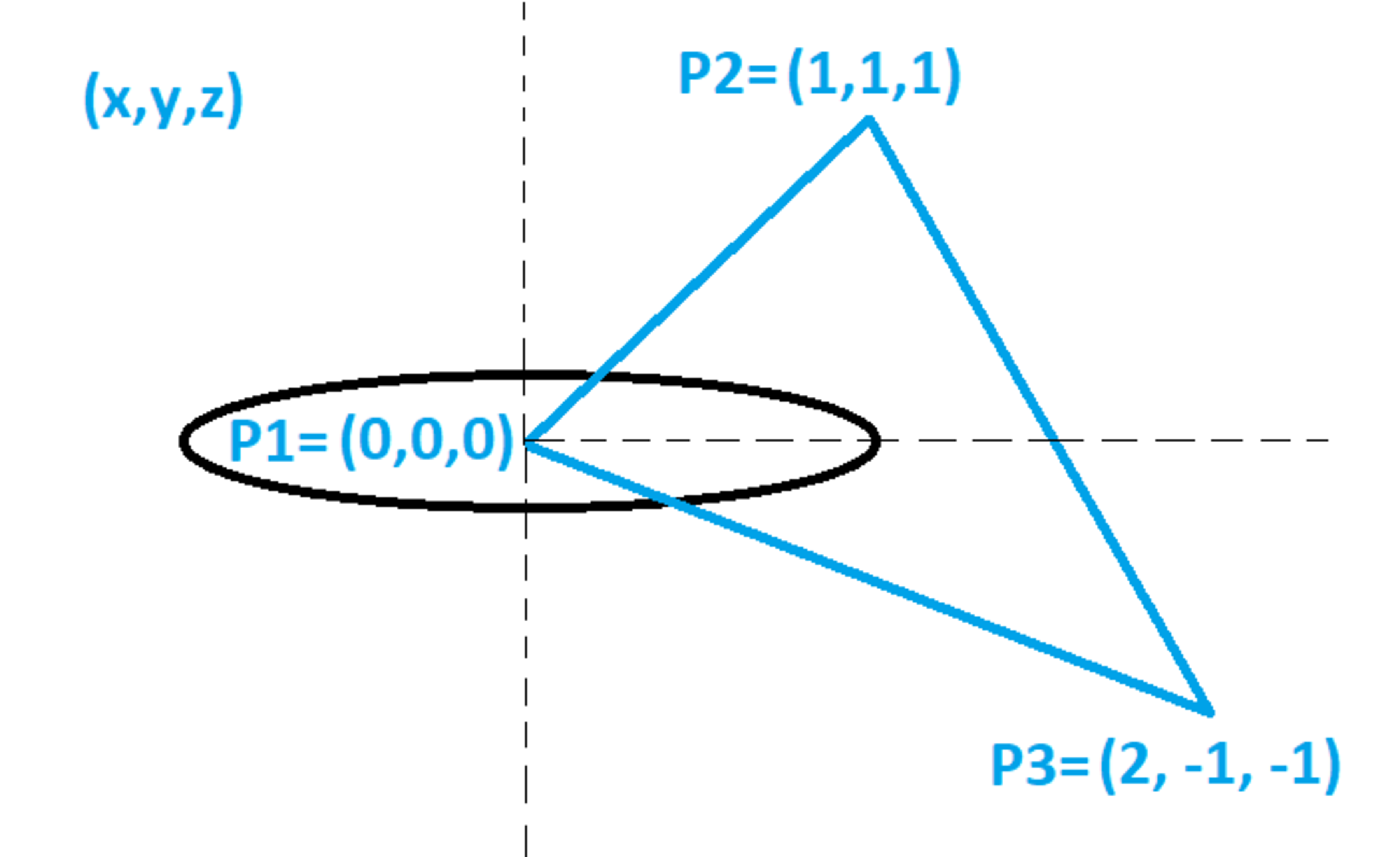
A circular wire loop of radius 1 lies within the x y plane and has its center at the origin. The loop carries 1 unit of electric current. A closed triangular loop has the vertices shown in the diagram. Consider the following three magnetic line integrals:
Q 1 2 = ∫ P 1 P 2 B ⋅ d ℓ Q 2 3 = ∫ P 2 P 3 B ⋅ d ℓ Q 3 1 = ∫ P 3 P 1 B ⋅ d ℓ
In the above integrals, B is the vector magnetic flux density produced by the loop at a particular point. Determine the following ratio:
Q 1 2 + Q 2 3 + Q 3 1 Q 1 2 Q 2 3 Q 3 1
Details and Assumptions:
1)
Magnetic permeability
μ
0
=
1
2)
You know ahead of time what the denominator of the ratio is
3)
All three
Q
values are positive
4)
All three integrals are evaluated along straight-line paths between points
The answer is 0.0159.
This section requires Javascript.
You are seeing this because something didn't load right. We suggest you, (a) try
refreshing the page, (b) enabling javascript if it is disabled on your browser and,
finally, (c)
loading the
non-javascript version of this page
. We're sorry about the hassle.
1 solution
@Karan Chatrath how you post this type of solution in this format is it computer language.? Sir can't you write solution simply sir please??
Log in to reply
Could you specify the difficulty you face a little more? Also, refer to the steps shown before the code. Those steps describe the process of calculation. I have followed those exact steps in the code. I suggest you compute the integrands by following the steps. You can construct expressions and solve the integrals using Wolfram, for instance.
Log in to reply
Bhaiya i face a lot of difficulty in this computer code language can you please write the whole solution
Log in to reply
@A Former Brilliant Member – Okay, I will update the solution. Computing and writing out explicit expressions takes me time so I will do that when I can. In the meantime, please tell me whether you can understand the steps I have shown before the code? You essentially need to follow those exact steps to construct the integrands.
Log in to reply
@Karan Chatrath – @Karan Chatrath how you parametrised that point in the first line of your solution I can't able to understand that sir please can you help?
Log in to reply
I hope that this helps. Enlarge the image while viewing it. I have added it to my solution as well.
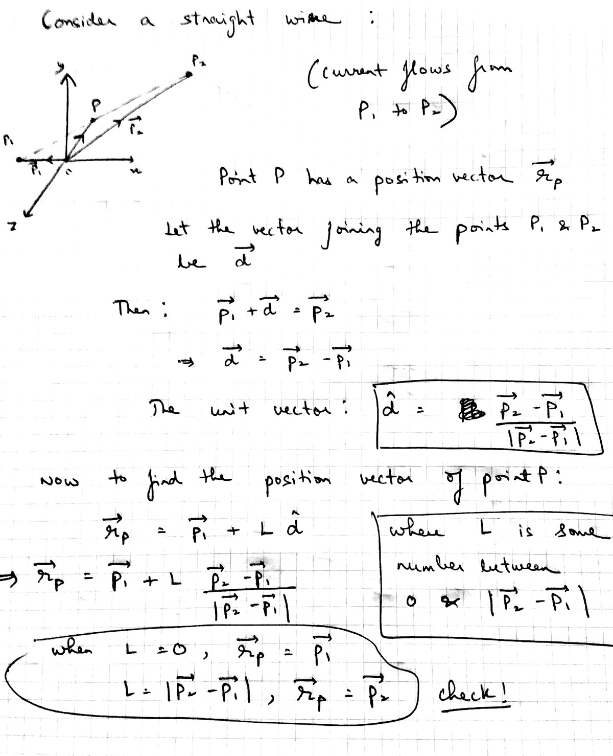
I shall show the line integral calculation steps for Q 1 2 .
Any point P on the line joining points P 1 and P 2 can be parameterised as follows:
r p = P 1 + L ∣ P 2 − P 1 ∣ P 2 − P 1
Where the parameter L varies from zero to a 1 = ∣ P 2 − P 1 ∣ . Any point on the circular loop can be parameterised using polar coordinates:
r c = cos θ i ^ + sin θ j ^
d r c = ( − sin θ i ^ + cos θ j ^ ) d θ
Applying Biot Savart law to obtain the field at point P on the line joining P 1 and P 2 gives:
d B 1 = 4 π μ o I ( ∣ r p − r c ∣ 3 d r c × ( r p − r c ) )
The total magnetic field at point P is, therefore:
B 1 = ∫ 0 2 π d B 1
A line element on the line joining points P 1 and P 2 is as follows:
d r p = d L ∣ P 2 − P 1 ∣ P 2 − P 1
The line integral is therefore:
Q 1 2 = ∫ 0 a 1 B 1 ⋅ d r p
This calculation is done using a simple script of code as follows. The other line integrals can follow the exact same procedure. Bear in mind the directions of current flow at all times.