Applied QM - Gaussian Potential
A particle in a one-dimensional quantum well is governed by a variant of the time-independent Schrodinger equation, expressed in terms of a non-normalized wave function Ψ N ( x ) .
The quantities V and E are the potential energy and total energy, respectively.
− d x 2 d 2 Ψ N ( x ) + V ( x ) Ψ N ( x ) = E Ψ N ( x )
The potential varies as follows:
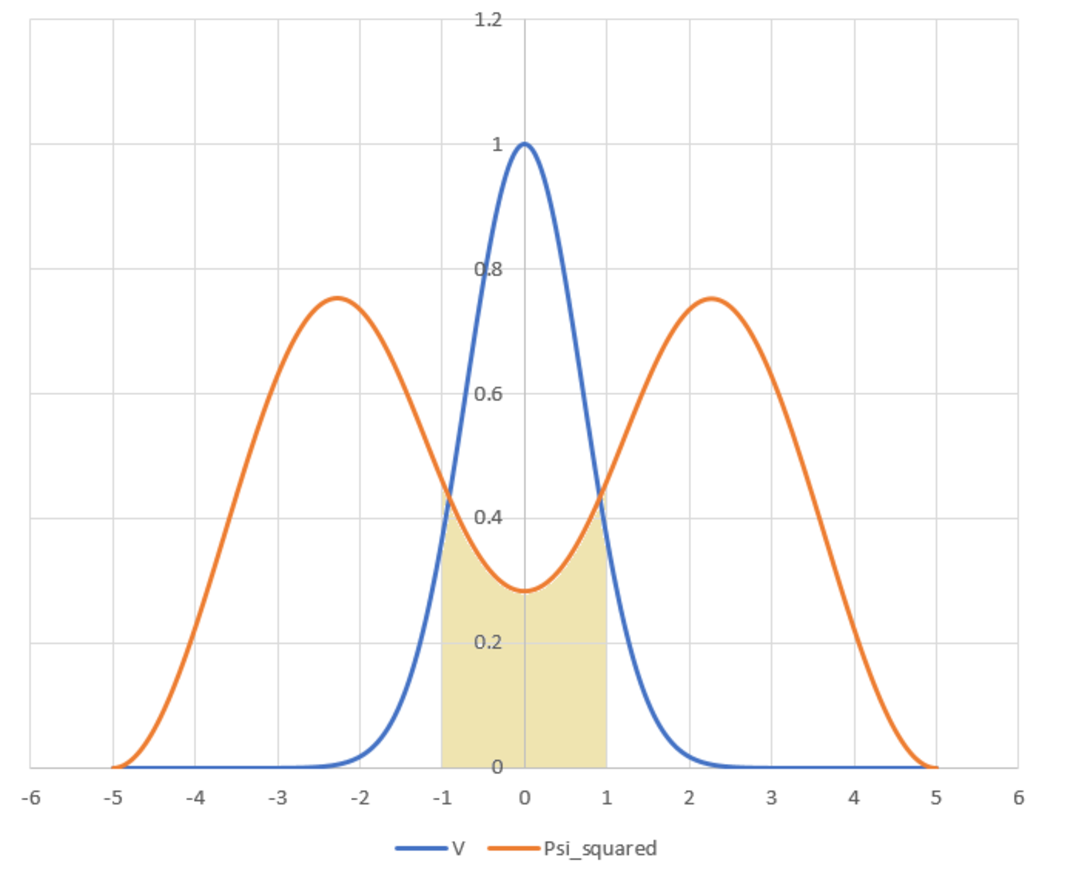
V ( x ) = ∞ x < − 5 V ( x ) = e − x 2 − 5 ≤ x ≤ 5 V ( x ) = ∞ x > 5
Consider the case in which E is at its smallest allowable value. What is the probability of detecting the particle in the region − 1 ≤ x ≤ 1 ?
Bonus: Based on the distribution of the wave function in relation to the potential function, what physical analogy can we make with classical mechanics?
The answer is 0.1575.
This section requires Javascript.
You are seeing this because something didn't load right. We suggest you, (a) try
refreshing the page, (b) enabling javascript if it is disabled on your browser and,
finally, (c)
loading the
non-javascript version of this page
. We're sorry about the hassle.
3 solutions
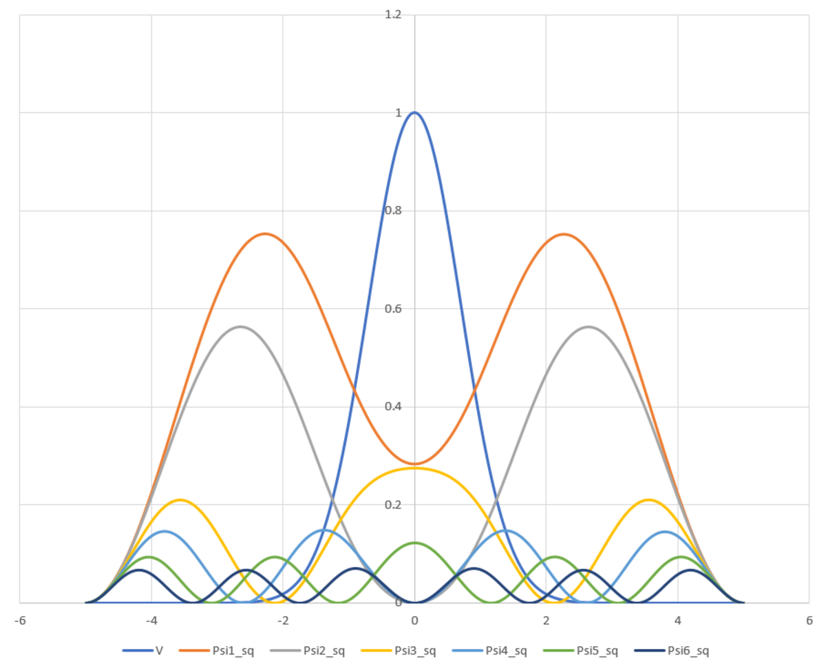
We have already seen some nice solutions by @Mark Hennings and @Karan Chatrath. The only thing I will add here is some plots for the higher-energy modes. The energies are as follows:
E 1 ≈ 0 . 3 3 2 E 2 ≈ 0 . 4 4 5 E 3 ≈ 1 . 1 8 9 E 4 ≈ 1 . 7 0 9 E 5 ≈ 2 . 6 8 4 E 6 ≈ 3 . 7 1 9
The first two modes "prefer" the low-potential regions, analogously with classical mechanics. From then on, the odd-numbered modes have a local maximum in the probability density coinciding with the potential peak, and the even-numbered modes do not.
Post-script :
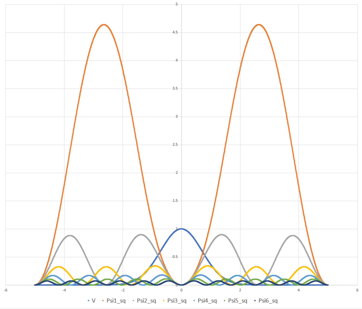
The energy levels above were found by imposing the boundary conditions Ψ ( − 5 ) = 0 and d x d Ψ ( − 5 ) = 0 . If we instead impose the conditions Ψ ( 0 ) = 0 and d x d Ψ ( 0 ) = 0 , we get another set of energies, some of which are basically in common with the first set. Notice that E 1 , E 2 , and E 3 from this set correspond to E 2 , E 4 , and E 6 from the other set. The probability density plots for these modes are given below. Notice that all of them now "avoid" the high potential region.
E 1 ≈ 0 . 4 4 5 E 2 ≈ 1 . 7 1 2 E 3 ≈ 3 . 7 2 5 E 4 ≈ 6 . 4 9 5 E 5 ≈ 1 0 . 0 4 8 E 6 ≈ 1 4 . 3 8 9
The potential is even, but you have only given even eigenstates. There should be odd ones as well. I am away from my computer at present, but if we put ψ ( 0 ) = 0 and ψ ′ ( 0 ) = 1 , are there values of E that give ψ ( 5 ) = 0 ?
My guess is that even and odd energy levels alternate...
Log in to reply
You are correct. I have added a post-script to the solution showing this. Thanks for the suggestion. @Karan Chatrath , you might be interested in this as well.
Log in to reply
@Steven Chase sir please can you upload the solution of your question 'planetary ballistics'. I am not able to solve. Please sir.
Log in to reply
@A Former Brilliant Member – I just numerically integrated to simulate the trajectory for various values of the initial velocity, and stopped when the initial velocity became sufficient to reach the equator.
So we can impose boundary conditions at the ends or in the middle, and we get a list of energies for each case, some of which coincide. Both are just subsets of the master list of allowed energies. In general, will the lowest energy correspond to end boundary conditions, or to middle boundary conditions? In this case, it corresponds to end boundary conditions.
@Mark Hennings , @Steven Chase , There is a gap in my understanding of QM here. When you call eigenstates odd or even, does it imply that the wave functions are odd or even functions? I ask this because the plots are of ψ 2 (which are even functions) and not ψ ( x ) itself. Looking at the wave functions only (and not the probability density function ψ 2 ), I would say that there are odd and even wave functions which alternate with increasing allowable energy levels. I hope I could explain my question clearly.
Log in to reply
Now that I am back at a computer, not a phone, I agree that the plots are of ψ 2 , and that (the squares of) both even and odd functions are there.
As Mark said, you can dictate the even-ness or odd-ness of the wave function by the boundary conditions:
1) For an even wave function, declare
Ψ
(
0
)
=
0
and
Ψ
′
(
0
)
=
0
2) For an odd wave function, declare
Ψ
(
0
)
=
0
and
Ψ
′
(
0
)
=
0
And then to find a master list of energy levels, perform the energy sweep once for each set of boundary conditions and combine the two sets of energies together.
End or middle does not matter. The Hamtonian commutes with the space reversal operator f ( x ) ↦ f ( − x ) , so there should be mutual eigenvectors of the Hamiltonian and space reversal - in other words, energy eigenstates that are either even or odd. We can solve for even ones with the initial conditions ψ = 1 and ψ ′ = 0 at x = 0 , solve the DE for 0 ≤ x ≤ 5 and defining the values for negative e x to suit. We can handle odd ones with the initial conditions ψ = 0 and ψ ′ = 1 at x = 0 , solving for 0 ≤ x ≤ 5 and making the function odd.
There should be odd eigenstates, or some reason why they don't exist... I get access to some calculations power again tomorrow, and will report back...
Log in to reply
@Mark Hennings sir can you upload the solution of the question( 'planetary ballistics' by Steven chase sir). I am not able to solve. Please sir
Log in to reply
Done. We have an exact solution... @Steven Chase
I have nothing new to add to the solution posted by @Mark Hennings, except that this is the first time I have used the Brilliant coding environment.
The differential equation can be re-written as a system of first order ODE's by taking y 1 ( x ) = ψ ( x ) and y 2 ( x ) = ψ ˙ ( x ) :
y ˙ 1 = y 2 y ˙ 2 = ( e − x 2 − E ) y 1
The dot notation denotes derivative with respect to x .
[ y ˙ 1 y ˙ 2 ] = [ y 2 ( e − x 2 − E ) y 1 ] y ˙ = f ( x , y )
It has been established in previous problems that the shape of the wave function is independent of the spatial derivative. So taking boundary conditions at x = − 5 as:
y ( − 5 ) = [ 0 1 ]
The system of ODE's is numerically integrated using the Euler step as such:
y ( k + 1 ) = y ( k ) + f ( x ( k ) , y ( k ) ) δ x
As x varies from -5 to 5. The value of energy E was incrementally increased until ψ ( 5 ) = 0 . This led to:
E = 0 . 3 3 1 8 5
The probability is computed as such:
P = ∫ − 5 5 ψ 2 ( x ) d x ∫ − 1 1 ψ 2 ( x ) d x
As for the bonus question, the wave function indicates that the particle is unlikely to be found near the area of maximum PE. This is because the region around the maximum corresponds to an unstable equilibrium. This is in line with classical mechanics.
Simulation code is as follows:
1 2 3 4 5 6 7 8 9 10 11 12 13 14 15 16 17 18 19 20 21 22 23 24 25 26 27 28 29 30 |
|
Greetings, and thanks for the solution. I typically just type three ticks (```) at the start and end, and put the code in the middle
Log in to reply
It is clearly a mess at the moment, as you might see.
Log in to reply
The ticks have to be on their own lines (not concatenated with the code text)
Log in to reply
@Steven Chase – Done, thanks!
@Steven Chase – I have also just included a comment on the bonus question. The solution is now complete. Thank you for the problem and for your help.
Log in to reply
@Karan Chatrath – Indeed, I was amused to see the particle "preferring" the low-potential regions. Nice to see something intuitive coming out of QM.
Log in to reply
@Steven Chase – This result is in line with intuition. But if you look at the problem on the sine potential, the result is contrary to what we now expect (unless I am doing or thinking something wrong). Thought-provoking..
Log in to reply
@Karan Chatrath – Interesting. I did the energy analysis on that one, but didn't actually look at the wave function graph. I would expect the sine one to be qualitatively similar to this one.
Log in to reply
@Steven Chase – I went back to that problem to check if the observation made here is consistent in different scenarios. Do look into it when you can.
Log in to reply
@Karan Chatrath – I looked at the sine problem again. For the lowest allowable energy, the peak probability density coincides with the potential peak, which is indeed counterintuitive. However, for the second smallest allowable energy, the probability density peaks resemble those seen in the Gaussian case.
@Karan Chatrath – I also tried several higher energies after that for the sine potential. Suppose E 1 is the lowest energy level. In general, the wave function for energy E n avoids the central potential peak for even values of n , and it has a peak coinciding with the potential peak for odd values of n .
Log in to reply
@Steven Chase – Thanks for sharing your observations. The point to be addressed now is the interpretation of the results. I will give it a thought
Log in to reply
@Karan Chatrath – @Karan Chatrath Sir can you upload the solution of the question( 'planetary ballistics' by Steven chase sir). I am not able to solve. Please sir
Log in to reply
@A Former Brilliant Member – I solved that problem using numerical integration. I will, however, post a solution when I can. I will specify the steps involved.
We are looking for solutions of the differential equation − y ′ ′ ( x ) + e − x 2 y ( x ) = E y ( x ) 0 ≤ x ≤ 5 with y ( 0 ) = 1 , y ′ ( 0 ) = 0 (the ground state will be an even function) and y ( 5 ) = 0 .
Solving the differential equation, with the initial conditions y ( 0 ) = 1 , y ′ ( 0 ) = 0 , numerically, we can solve numerically to find the smallest positive value of E that gives y ( 5 ) = 0 ; this is E = 0 . 3 3 1 8 7 4 0 7 1 .
For this value of E , we then calculate ∫ 0 5 y ( x ) 2 d x ∫ 0 1 y ( x ) 2 d x = 0 . 1 5 7 4 4 7 for the required probability.