Curly Trajectory
At time t = 0 , a particle of mass 1 in the ( x , y ) plane has the following position and velocity:
( x , y ) = ( 0 , 0 ) ( x ˙ , y ˙ ) = ( 1 5 , 1 0 )
The particle experiences the following force:
F = ( F x , F y ) = ( − 3 0 y ˙ sin ( t ) , 3 0 x ˙ sin ( t ) )
How far from the origin is the particle at t = 1 2 ?
The answer is 16.98.
This section requires Javascript.
You are seeing this because something didn't load right. We suggest you, (a) try
refreshing the page, (b) enabling javascript if it is disabled on your browser and,
finally, (c)
loading the
non-javascript version of this page
. We're sorry about the hassle.
4 solutions
Interesting. I used explicit Euler and it converged reasonably nicely. I used timesteps of 1 0 − 5 , 1 0 − 6 , and 1 0 − 7 . The difference between the 1 0 − 6 result and the 1 0 − 7 was negligible
Log in to reply
How come your explicit Euler converged reasonably? I implemented pretty much the exact same code as you, and found for timestep 1 0 − 5 it was very inaccurate. Only 1 0 − 7 actually produced 16.98, as opposed to 16.99, which 1 0 − 6 produces. By the way, the code takes about 10 seconds to run for a 1 0 − 6 timestep despite my great computer processor.
Log in to reply
I think the only difference is how we define "reasonably nicely". In my opinion, your results for 1 0 − 5 , 1 0 − 6 , 1 0 − 7 show acceptable convergence
Well, that would have saved some time! I must have made a mistake in my implementation.
Still, I was very surprised the analytical solution at least partly worked.
How did you come up with this system? (Oh, and what did you use to plot the trajectory?)
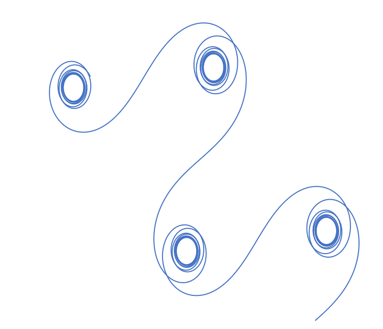
I got interested in generating random smooth curves from physics principles some time ago (see the linked note). This is basically just a slightly better-behaved version of that. I just use Python to spit out the (x,y) coordinates, and then I plot as an (x,y) scatter in Excel.
https://brilliant.org/discussions/thread/generating-random-smooth-curves-using-physics/
Log in to reply
That's awesome - thanks for sharing. Looks like I really missed the point trying for an analytical solution! Would you mind posting your Python code for this one? (I did my coding using VBA, of all things!)
Log in to reply
I posted the Python code as a solution. I did some "Hello World"-level stuff in highschool with Visual Basic, but didn't do any math in it. Is it easy to use for math calculations?
Log in to reply
@Steven Chase – VBA is easy to use in general, if you grew up coding BASIC-style languages (as I did), but it's not really designed for maths calculations in the way that Python and its modules are (eg no vector handling). It's also not as efficient in terms of runtime - that's what put me off step sizes of 10^-7, whereas, of course, what I should be doing is learning Python (to that end, thank you for your code!)
Where VBA in Excel can be useful is manipulating objects in Excel, though, so occasionally I'll use it for constructing diagrams.
Simulation code (Python). This uses explicit Euler integration with a very small time step.
1 2 3 4 5 6 7 8 9 10 11 12 13 14 15 16 17 18 19 20 21 22 23 24 25 26 27 28 29 30 31 32 33 |
|
I do not have any solution to add to this problem. Even I solved it numerically. I was just playing around with the initial conditions and I was surprised to see the genesis of some very beautiful looking solutions. I have attached a screenshot.
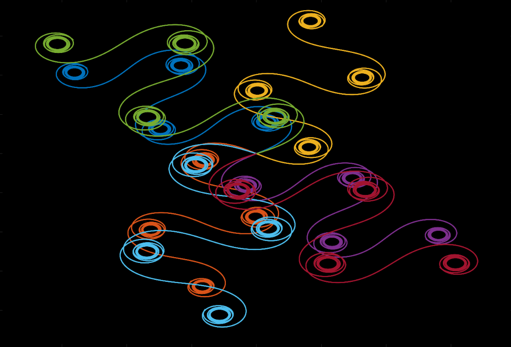
What I find really remarkable is that solving a simple set of equations can yield such patterns. There is indeed beauty hidden in mathematics. Maybe this tells us more than what we can appreciate with our current state of knowledge. Good examples of such patterns are the Lorenz strange attractor and the Mandelbrot set.
As always, a very nice problem!
That's really cool. It could be an art piece in somebody's house. I can't draw, but I have made some fairly nice math art before.
Log in to reply
Yes, I saw the link you posted on random smooth curves. I will go through it soon. Thanks!
Very pretty! I'd point out, though, that this is not exhibiting chaotic behaviour like the Mandelbrot set or Lorenz attractor (which is itself perhaps a little surprising at first, though there are good reasons for this). If you look carefully you'll see the plotted curves are all rotations and translations of each other.
That is a good point. The system here, unlike the examples I gave is not chaotic. Mainly because the given dynamical system is linear. One of many pre requisites for a chaotic system is non-linearity. Thank you for sharing the link.
Beautiful renderings!
Here is my code, which uses Explicit Euler Integration. Given the nature of the differential equations that describe the system, I don't think Explicit Euler is the best method. The code is actually pretty inaccurate for even slightly greater timesteps; the timestep which will yield a satisfactory result is 1 0 − 6 . It needs hardware acceleration; CUDA python is the best way to go. At the end of the code, the results are shown at various values of deltaT, as are the times taken to compile the code at the values of deltaT.
The code takes a long time to compile as the step size increases. The error in the result is dependent on step size. The Euler method is inaccurate and the convergence of the result is very slow. It is also very time consuming to compute such small values of deltaT on the CPU, and get an inaccurate result nevertheless. A better method which has O ( n 4 ) error would be Runge-Kutta.
Edit: I have tried it with a modified Euler technique below as well:
1 2 3 4 5 6 7 8 9 10 11 12 13 14 15 16 17 18 19 20 21 22 23 24 25 26 27 28 29 30 31 32 33 34 35 36 37 38 39 40 41 42 43 44 45 46 47 48 49 50 51 52 53 54 55 |
|
It's convenient to rewrite the system as follows:
x ˙ = u
y ˙ = v
u ˙ = − 3 0 v sin t
v ˙ = 3 0 u sin t
subject to the initial conditions x ( 0 ) = y ( 0 ) = 0 , u ( 0 ) = 1 5 , v ( 0 ) = 1 0 .
Although we've introduced more variables, making the system larger, it is now first order, and easier to handle. Note that the sub-system in u and v is entirely self-contained; we can solve for ( u , v ) first, then integrate to find ( x , y ) .
I tried a few approaches to this.
This felt like a well-devised trap that I fell into. The method fails, terribly, even for very small step sizes.
[Edit: turns out, this wasn't a trap at all and should have worked - see the comments below]
This worked better, though still needed small step sizes to work. The scheme is as follows:
r k + 1 = ( I − h A k + 1 ) − 1 r k
where r k = ( u k v k ) , A k = ( 0 3 0 sin t k − 3 0 sin t k 0 ) , t k = k h , and h is the step-size. This is not as bad to implement as I made it look!
Once the u and v values were calculated up to t = 1 2 , I just used numerical integration to get x and y (the position of the particle after this time).
The results for a few h -values are below:
These values seem to be converging, but slowly. Quite a handy trick here is to extrapolate from these data points using the ratio of the differences in the successive answers. Using this gave an estimate of 1 6 . 9 7 8 7 5 … for the answer.
And this is what I should have done first. Going back to the system of equations, we have
u ˙ = − 3 0 v sin t
v ˙ = 3 0 u sin t
Dividing through, v ˙ u ˙ = − u v
Simplifying, u ˙ u + v ˙ v = 0
so that u 2 + v 2 = const.
From the initial values, the constant is 3 2 5 .
We can now substitute v = 3 2 5 − u 2 to give
u ˙ = − 3 0 3 2 5 − u 2 sin t , which is a separable equation. With the initial condition u ( 0 ) = 1 5 , the solution is
u ( t ) = − 5 1 3 sin ( − 3 0 cos ( t ) + 3 0 − sin − 1 ( 1 3 3 ) )
Likewise, v ( t ) = 5 1 3 sin ( − 3 0 cos ( t ) + 3 0 + sin − 1 ( 1 3 2 ) )
Integrating these numerically, we find that x ( 1 2 ) = − 1 3 . 0 5 0 5 … and y ( 1 2 ) = 1 0 . 8 6 1 … , giving the particle's distance from the origin as 1 6 . 9 7 8 7 … .