Magnetism+Viscosity+Rotation
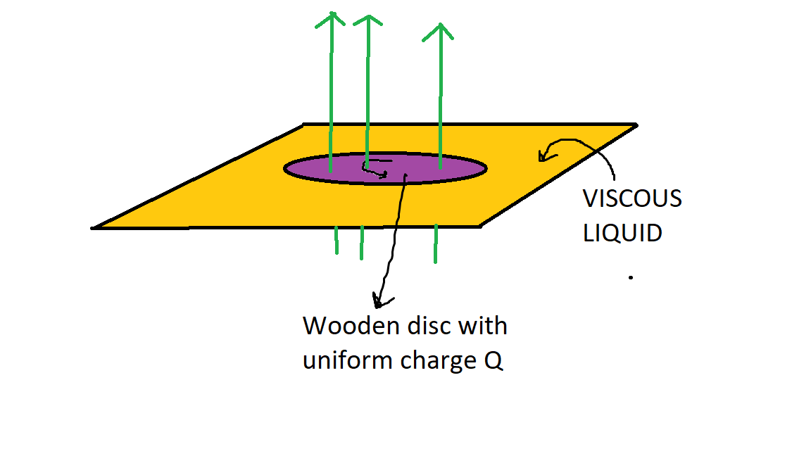
There is a non-conducting, viscous liquid(Yellow colour). A uniformly charged non conducting wooden disc of mass M and radius R is kept over the thick viscous liquid where the thickness of the liquid is d . The scientist wants to know the coefficient of viscosity of the liquid. So he devises this method. He uses a magnetic field where the magnetic field varies with time as B = b t where b is a constant. (Green lines are the magnetic field lines). Now he sets the value of b in such a way that the disc keeps on rotating with constant angular velocity ω 0 .
This was his setup. (Although his setup is quite big and nonsensical, still he uses it to find out the coefficient of viscosity).
Find out the value of coefficient of viscosity with the following data and assumptions.(in SI Unit)
Values
-
Q = π C
-
b = 2 T / s
-
ω 0 = 1 0 r a d / s
-
R = 2 m
-
M = 2 k g
-
d = 2 m
Details And Assumptions
-
Consider that magnetic field is everywhere over the disc.
-
Consider that the liquid has no effect while applying magnetic field.
-
Consider that the disc to be placed over the liquid.
-
Completely original (Made in my dream)
-
Consider coefficient of friction between disc and liquid to be 0.(The one which occurs due to Normal Reaction)
The answer is 0.05.
This section requires Javascript.
You are seeing this because something didn't load right. We suggest you, (a) try
refreshing the page, (b) enabling javascript if it is disabled on your browser and,
finally, (c)
loading the
non-javascript version of this page
. We're sorry about the hassle.
1 solution
Nice!! I always tend to make silly errors :P
I posted one today which is inspired by this one
Log in to reply
Yeah sir. Solved it. Interesting it was!! Liked solving it
https://brilliant.org/problems/computational-physics-mechanical-system/
How do we do this with CS?
Log in to reply
There are eight unknowns and eight equilibrium equations (two for each joint). It is therefore an 8x8 linear algebra problem. I have posted a solution under that problem. Long story short, the problem has nothing to do with CS, but it was placed under CS because a computer solution is the most convenient way to do it.
Log in to reply
@Steven Chase – Tha ks sir for clearing out my doubt.
Sir, need hints for this. https://brilliant.org/problems/gravitational-collapse/ Thanks
Log in to reply
I solved it with numerical integration. Are you familiar with that?
Log in to reply
@Steven Chase – I mean can you tell me the concept involved. Did you understand what i mean? And how y varies with x at any time and all...
If you used different method, You may tell me that. Numerical integration is like this isnt it?
https://drive.google.com/file/d/1I_RTShxXHRhBJNxea3dzrxWrBEv7LIip/view?usp=sharing
Log in to reply
@Md Zuhair – The beauty of numerical integration is that you don't have to have a closed form expression for the relationships between variables. You just compute the changes step by step. For example, consider the variable x, its first time derivative, and its second time derivative. Let's say that the subscript "k" denotes the present processing interval, and the subscript "k-1" denotes the previous processing interval. Euler integration looks like this:
x k = x k − 1 + x ˙ k − 1 Δ t x ˙ k = x ˙ k − 1 + x ¨ k − 1 Δ t x ¨ k = f ( x , . . . . . )
Log in to reply
@Steven Chase – Dont we do it like this sir? https://drive.google.com/file/d/1I_RTShxXHRhBJNxea3dzrxWrBEv7LIip/view?usp=sharing
Log in to reply
@Md Zuhair – Yeah, that's it. Except here, we have variation over time, and multiple derivatives, and multiple quantities changing.
Log in to reply
@Steven Chase – Yeah... true.. I see... Thanks sir. But how do we apply in the question?
Log in to reply
@Md Zuhair – Here is my code. I re-wrote it just now, since the problem is so old. The random numbers are just to ensure that the result is independent of the particular values of the constants.
1 2 3 4 5 6 7 8 9 10 11 12 13 14 15 16 17 18 19 20 21 22 23 24 25 26 27 28 29 30 31 32 33 34 35 36 37 38 39 40 41 42 43 |
|
Log in to reply
@Steven Chase – Is this python sir?
Log in to reply
@Md Zuhair – Yes, it is
Log in to reply
@Steven Chase – Oh,we are taught C++ . Still I can understand what it means. Thank you sir for you precious time. Have a nice day. Here its almost 2 AM at night. Good Night.
Log in to reply
@Md Zuhair – Sure thing. I also learned on C++ to begin with, but I now use Python. Talk to you later.
Hello sir, how are you doing? Remember me?
Log in to reply
Hello. Yes, I do indeed. Things are a bit crazy these days, but I'm doing fine. Still posting lots of problems. How about you?
Log in to reply
@Steven Chase – Nice to learn that sir. Sir Im now pursuing computer engineering at one of the eminent institutes in India named IIT. Please keep posting your qs, they are pretty awesome! Things are bit crazy in brilliant or your personal life?
The fluid shear drag torque should be equal to the electric torque. This whole problem consists of analyzing the contributions from infinitesimal concentric rings.
Begin fluid portion
Infinitesimal fluid shear force and torque:
d F = μ d A d v = μ 2 π r d r d r ω 0 = d 2 π ω 0 μ r 2 d r d τ = d F r = d 2 π ω 0 μ r 3 d r
Total fluid shear torque
τ = ∫ 0 R d 2 π ω 0 μ r 3 d r = 4 d 2 π ω 0 μ R 4 = 2 d π ω 0 μ R 4
End fluid portion
Begin electric portion
Flux linkage for loop of radius r:
λ = π r 2 B = π r 2 b t
Voltage for loop of radius r:
ϵ = λ ˙ = π r 2 b
Electric field at radius r:
E = 2 π r ϵ = 2 1 r b
Infinitesimal charge at radius r:
d Q = Q π R 2 2 π r d r = R 2 2 Q r d r
Infinitesimal force at radius r:
d F = E d Q = R 2 Q b r 2 d r
Infinitesimal torque at radius r:
d τ = r d F = R 2 Q b r 3 d r
Total electric torque:
τ = ∫ 0 R R 2 Q b r 3 d r = 4 Q b R 2
End electric portion
Setting torques equal
2 d π ω 0 μ R 4 = 4 Q b R 2 μ = 4 π ω 0 R 4 2 d Q b R 2 = 2 π ω 0 R 2 d Q b = 2 π × 1 0 × 4 2 × π × 2 = 0 . 0 5