No SHM here

Classical Mechanics Level 4

Difficulty: Moderate.

A pendulum hinged at the origin of point-mass $m = 1kg$ with string length $l = 1m$ is dropped from an angle $\displaystyle \theta = \frac{1}{2} \pi$ radians, with respect to the negative $y$ -axis (see below for the coordinate system) .

However, this time, there is basic drag force, dependent on the velocity of the point-mass, given by:

$\displaystyle \vec{\bold{F}}_{d} = -C_{drag} l \dot{\theta}$

This drag force opposes the motion of the mass.

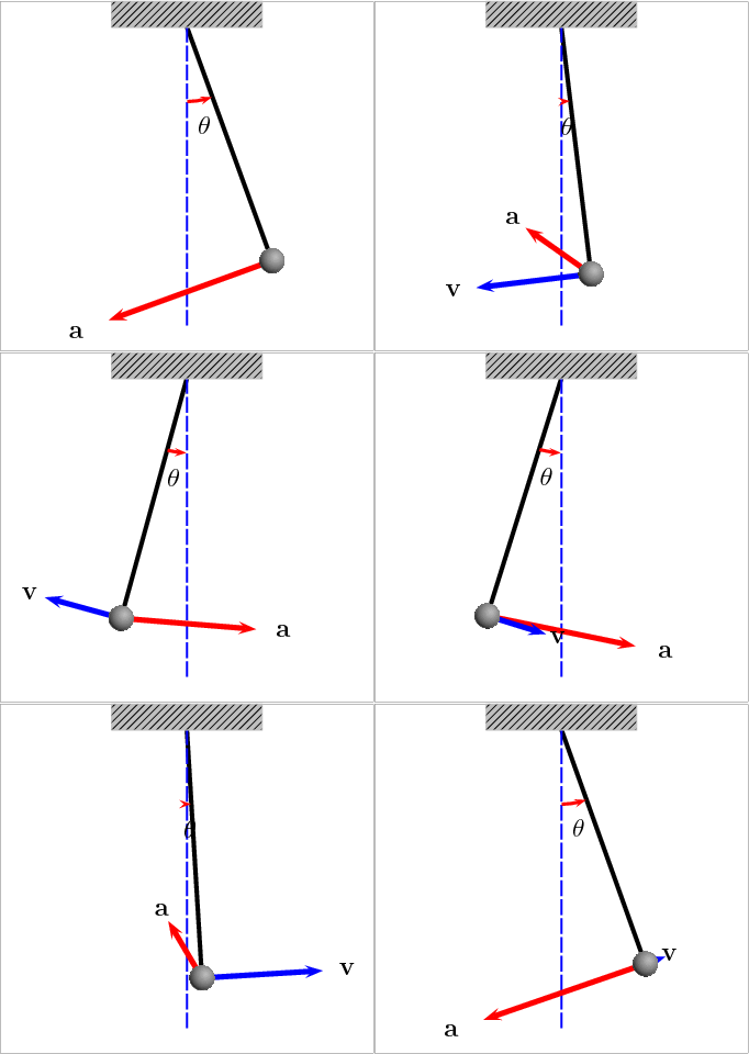
Find the time it takes for the bob to reach $x = 0$ or $\theta = 0$ , after the bob swings fully to the left . In other words, find the time it takes for the second instance where the bob reaches $\theta = 0$ . Enter your answer in seconds to 1 decimal place.

Try to use numerical methods to solve; integrals will not help you here due to the complexity of the EOM.

Note:

Here gravity is in the negative $y$ direction, and equal to $10 m/s^2$
$C_{drag} = 1$
$\dot{\theta}$ is the first derivative with respect to time of $\theta$
see how $\theta$ is defined in the GIF above

The answer is 1.69.

2 solutions

Krishna Karthik
May 24, 2020

Edit: it seems there was a slight miscalculation in my program, and when originally entering the answer, I accidentally set time-step to $10^{-2}$ , something which was left over from graphing. I rechecked, and the more precise answer is 1.714826 seconds

I'm going to use the Newtonian model to derive the equation of motion, although this can be done the Lagrangian way, by introducing a dissipative term into the Euler-Lagrange equation. The maths is harder by Lagrangian, however:

$\displaystyle \frac{d}{dt} \frac{ \partial L}{\partial \dot x} = \frac{ \partial L}{\partial x} + \frac{ \partial D}{\partial x}$

The force of gravity acting on the particle tangentially is:

$\displaystyle \bold{F_{tangential}} = -mg \sin(\theta)$

The force of drag acting opposite to $\dot{\theta}$ is:

$\displaystyle \bold{F_d} = -l \dot{\theta}$

Total force:

$\displaystyle m \ddot{\theta} = -mg \sin(\theta) - c \dot{\theta}$

I numerically integrated this till time $t = 10$ seconds, and plotted $\theta$ and time values.

The dampening force is acting well, and it looks realistic. The amplitude of each swing reduces due to drag; the dissipated energy increases after each swing. Here's an energy statistics graph:

I plotted with time-step $10^{-2}$ , but used Runge-Kutta 4th Order, which is more ideal for oscillating motion.

Here's my code (time-step $10^{-6}$ ):

#4th order Runge-Kutta numerical solution of second order ODE
import math
#initialisation


time = 0
deltaT = 10**-6
times = 0

length = 1
g = 10

c = 1
m = 1

angles = []
finalTime = 0



u_1 = 0.5*math.pi
u_2 = 0

def differentialEquation(t,x,xdot):  #applying RK4 by splitting 2nd order ODE into 2 first order ODEs
    return -g*math.sin(x)-(c/m)*(length*xdot)


print("times where x == 0: ")
print("")

while u_2 <= 0:

    #evaluating slope at various points

    k0 = deltaT*u_2
    L0 = deltaT*differentialEquation(time,u_1,u_2)

    k1 = deltaT*(u_2 + 0.5*L0)
    L1 = deltaT*differentialEquation(time + 0.5*deltaT, u_1 + 0.5*k0, u_2 + 0.5*L0)

    k2 = deltaT*(u_2 + 0.5*L1)
    L2 = deltaT*differentialEquation(time + 0.5*deltaT, u_1 + 0.5*k1, u_2 + 0.5*L1)

    k3 = deltaT*(u_2 + L2)
    L3 = deltaT*differentialEquation(time + deltaT, u_1 + k2, u_2 + L2)
    #RK4 approximation of values

    u_1 = u_1 + (1/6)*(k0 + 2*k1 + 2*k2 + k3)
    u_2 = u_2 + (1/6)*(L0 + 2*L1 + 2*L2 + L3)


    time += deltaT

finalTime = finalTime + time


time = 0

while u_1 <= 0:

    #evaluating slope at various points

    k0 = deltaT*u_2
    L0 = deltaT*differentialEquation(time,u_1,u_2)

    k1 = deltaT*(u_2 + 0.5*L0)
    L1 = deltaT*differentialEquation(time + 0.5*deltaT, u_1 + 0.5*k0, u_2 + 0.5*L0)

    k2 = deltaT*(u_2 + 0.5*L1)
    L2 = deltaT*differentialEquation(time + 0.5*deltaT, u_1 + 0.5*k1, u_2 + 0.5*L1)

    k3 = deltaT*(u_2 + L2)
    L3 = deltaT*differentialEquation(time + deltaT, u_1 + k2, u_2 + L2)
    #RK4 approximation of values

    u_1 = u_1 + (1/6)*(k0 + 2*k1 + 2*k2 + k3)
    u_2 = u_2 + (1/6)*(L0 + 2*L1 + 2*L2 + L3)


    time += deltaT


finalTime = finalTime + time

print("time : " +str(finalTime))

#result: 1.714826

Steven Chase
May 24, 2020

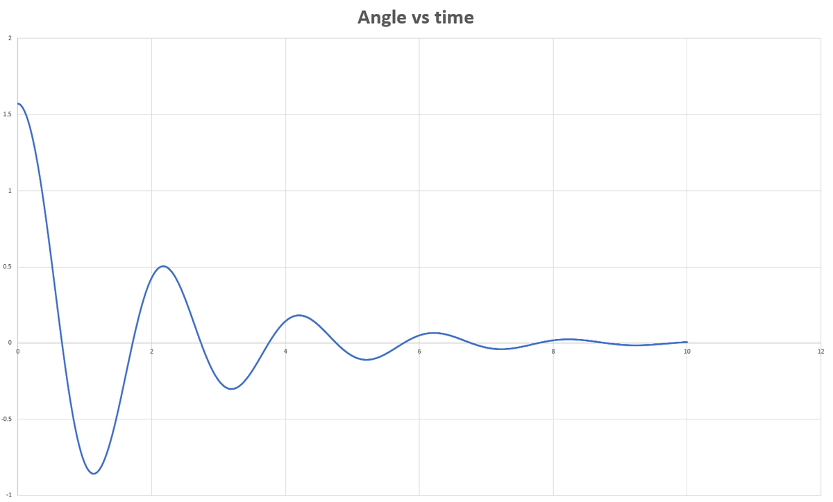
This was a fun problem. I divided the simulation into different time periods to keep track of how long each part takes. It takes the pendulum $\approx 0.660$ seconds to swing from its starting position to $\theta = 0$ . Then from the extreme left position, it takes $\approx 0.582$ seconds to move back to $\theta = 0$ . Relative to the very start of the simulation, the pendulum crosses $\theta = 0$ from the left at time $t \approx 1.7148$ . This differs slightly from the expected answer. I used explicit Euler with time steps of $10^{-5}$ and $10^{-6}$ . I have attached a graph of angle vs time as well.

import math

m = 1.0
L = 1.0
theta0 = math.pi/2.0
Cdrag = 1.0
g = 10.0

dt = 10.0**(-5.0)

I = m*(L**2.0)

################################

t = 0.0
count = 0

theta = theta0
thetad = -10.0**(-6.0)
thetadd = 0.0

while theta >= 0.0:

    theta = theta + thetad*dt
    thetad = thetad + thetadd*dt

    x = L*math.sin(theta)
    y = -L*math.cos(theta)

    xd = L*math.cos(theta)*thetad
    yd = L*math.sin(theta)*thetad

    v = math.hypot(xd,yd)

    ux = xd/v
    uy = yd/v

    rx = x
    ry = y

    Fgx = 0.0
    Fgy = -m*g

    Fdx = -Cdrag*v*ux
    Fdy = -Cdrag*v*uy

    Fx = Fgx + Fdx
    Fy = Fgy + Fdy

    Tau = rx*Fy - ry*Fx

    thetadd = Tau/I

    t = t + dt
    count = count + 1

    #if count % 1000 == 0:
        #print t,theta

t1 = t

################################

while thetad <= 0.0:

    theta = theta + thetad*dt
    thetad = thetad + thetadd*dt

    x = L*math.sin(theta)
    y = -L*math.cos(theta)

    xd = L*math.cos(theta)*thetad
    yd = L*math.sin(theta)*thetad

    v = math.hypot(xd,yd)

    ux = xd/v
    uy = yd/v

    rx = x
    ry = y

    Fgx = 0.0
    Fgy = -m*g

    Fdx = -Cdrag*v*ux
    Fdy = -Cdrag*v*uy

    Fx = Fgx + Fdx
    Fy = Fgy + Fdy

    Tau = rx*Fy - ry*Fx

    thetadd = Tau/I

    t = t + dt
    count = count + 1

    #if count % 1000 == 0:
        #print t,theta

t2 = t

################################

while theta <= 0.0:

    theta = theta + thetad*dt
    thetad = thetad + thetadd*dt

    x = L*math.sin(theta)
    y = -L*math.cos(theta)

    xd = L*math.cos(theta)*thetad
    yd = L*math.sin(theta)*thetad

    v = math.hypot(xd,yd)

    ux = xd/v
    uy = yd/v

    rx = x
    ry = y

    Fgx = 0.0
    Fgy = -m*g

    Fdx = -Cdrag*v*ux
    Fdy = -Cdrag*v*uy

    Fx = Fgx + Fdx
    Fy = Fgy + Fdy

    Tau = rx*Fy - ry*Fx

    thetadd = Tau/I

    t = t + dt
    count = count + 1

    #if count % 1000 == 0:
        #print t,theta

t3 = t

################################

while t <= 10.0:

    theta = theta + thetad*dt
    thetad = thetad + thetadd*dt

    x = L*math.sin(theta)
    y = -L*math.cos(theta)

    xd = L*math.cos(theta)*thetad
    yd = L*math.sin(theta)*thetad

    v = math.hypot(xd,yd)

    ux = xd/v
    uy = yd/v

    rx = x
    ry = y

    Fgx = 0.0
    Fgy = -m*g

    Fdx = -Cdrag*v*ux
    Fdy = -Cdrag*v*uy

    Fx = Fgx + Fdx
    Fy = Fgy + Fdy

    Tau = rx*Fy - ry*Fx

    thetadd = Tau/I

    t = t + dt
    count = count + 1

    #if count % 1000 == 0:
        #print t,theta


################################

print ""
print "#######################"
print ""
print dt
print ""
print t1
print t2
print t3
print ""
print (t3-t2)


#######################

#1e-05

#0.65993
#1.13276
#1.71484

#0.582080000004
#>>> 
#######################

#1e-06

#0.659920999998
#1.132745
#1.71482699995

#0.582081999952
#>>>

Woah that's so cool how you produced nearly the exact same graph as me. They look so similar. I like how you directly simulated by calculating force at each point rather than simply numerically integrating the EOM. I may use that approach in some of my upcoming problems!

Krishna Karthik - 1 year ago

I wonder... maybe the difference in integration method caused the slight difference. Either-way, the graphs both show the exact same results. Thanks for posting the solution.

Krishna Karthik - 1 year ago

What result do you get when you use a time step of $10^{-5}$ or $10^{-6}$ ?

Steven Chase - 1 year ago

I get around 1.69 (converging to 1.7)

Krishna Karthik - 1 year ago

@Krishna Karthik – I suspect that there is some other slight discrepancy in how we are doing calculations. Because with time steps that small, both integration methods should agree very closely. But the results are close enough for me. Thanks for posting

Steven Chase - 1 year ago

@Steven Chase – Oh I rechecked, and it seems there is a slight discrepancy in my code, that made it less accurate originally when . The timestep (when ran the program) was $10^{-2}$ when I thought it was $10^{-6}$ , and clearly isn't small enough. I re-ran and put in $10^{-6}$ , which gives me the exact same answer as you, to 4 decimal places.

Well, I would update the solution if I could, but it won't allow. Since you have entered the exact answer and it did mark you as a solver, I hope there will be no problem for future solvers...

Krishna Karthik - 1 year ago

@Krishna Karthik – Brilliant's decimal answer format counts an attempt correct if it is within 3 percent of the expected answer. So it should be OK

Steven Chase - 1 year ago

No SHM here

The answer is 1.69.

2 solutions

0 pending reports