Ramp Potential - Energy Quantization

Classical Mechanics Level 5

This is a followup to the previous problem (see details there). For energy $E_1 = 2.5$ , the non-normalized wavefunction $\Psi_N (x)$ has the following properties:

$\Psi_N (0) = 0 \\ \Psi_N (x_f) = 0 \\ \Big ( \frac{d}{dx} \, \Psi_N \Big ) (0) = 1 \\ x_f \approx 3.0267 \, \text{(a zero crossing of } \Psi_N (x))$

Let $E_2$ be the smallest value of $E$ that is bigger than $E_1$ , such that the above conditions are true. What is the value of $E_2$ ?

The answer is 5.848.

2 solutions

Karan Chatrath
Aug 21, 2019

The solution of the differential equation was obtained numerically. In fact, I see these set of problems as a good opportunity to learn and eventually get comfortable with programming in the Brilliant coding-environment. I will post a solution later, for the previous problem using that. Here, I have simply increased the value of energy until the conditions are satisfied. It is an approach of trial and error. I did not just do this for $E_2$ . I computed the quantized energy levels until $E_7$ . The following are some plots.

That's a very nice graph, thanks. For the classic infinite potential well (with zero potential inside), $E_2$ is four times the value of $E_1$ . That is certainly not the case here. My approach with these well problems is to declare the wave function properties at one edge of the well, integrate it out until it has a zero crossing, and then put the other edge of the well there. I was curious to see whether or not this actually yielded energy quantization; hence this problem. On another note, if we had said that the spatial derivative at one end was one half instead of one, there presumably would have been an entirely different discrete set of energy levels.

Steven Chase - 1 year, 9 months ago

I was just testing out the last sentence of your comment out of curiosity. I just made an interesting observation. Turns out that the quantized energy levels are independent of the spatial derivative at $x = 0$ . I am thinking of how to interpret this.

Karan Chatrath - 1 year, 9 months ago

Fascinating, and contrary to my intuition. I guess the next question is: For a particular energy level, does the initial spatial derivative have any impact on the probability of locating the particle within a certain region?

Steven Chase - 1 year, 9 months ago

@Steven Chase – The answer to the question, as I see it, is no. I repeated the previous exercise that you posted with different values for the initial derivative and I still obtain the same answer.

Karan Chatrath - 1 year, 9 months ago

@Karan Chatrath – Yes, I got the same result. So the energy levels are dictated entirely by the well itself. And there are many different wavefunctions for a particular energy, all yielding the same "physics". So is "physics" defined by the wave function, or merely by the things that can be observed experimentally? This reminds me of electromagnetism, in which there are infinitely many pairs of the electric potential and vector magnetic potential which yield the same electric and magnetic fields. There is a discussion of that under the "Classical Gauge Theory" section of the attached link:

https://en.wikipedia.org/wiki/Gauge_theory

Steven Chase - 1 year, 9 months ago

@Steven Chase – Yes, this is the logical conclusion. Nice problems, by the way.

Karan Chatrath - 1 year, 9 months ago

@Karan Chatrath – Thanks. I was heavily editing that comment until your most recent reply. It's about three times as long now

Steven Chase - 1 year, 9 months ago

@Steven Chase – Thanks for sharing the link

Karan Chatrath - 1 year, 9 months ago

In hindsight, I should have remembered that the time-independent SE is an eigenvalue equation, much like what we have seen from linear algebra:

$\large{ \hat{H} \Psi = E \Psi}$

The energy values are the eigenvalues of the Hamiltonian operator, which contains the potential function. So it makes sense for them to be wholly defined (albeit implicitly) by the Hamiltonian.

Steven Chase - 1 year, 9 months ago

And hence independent of initial conditions imposed on the wave function.

Karan Chatrath - 1 year, 9 months ago

Do you use Matlab primarily?

Steven Chase - 1 year, 9 months ago

Yes, I do use Matlab.

Karan Chatrath - 1 year, 9 months ago

Steven Chase
Aug 21, 2019

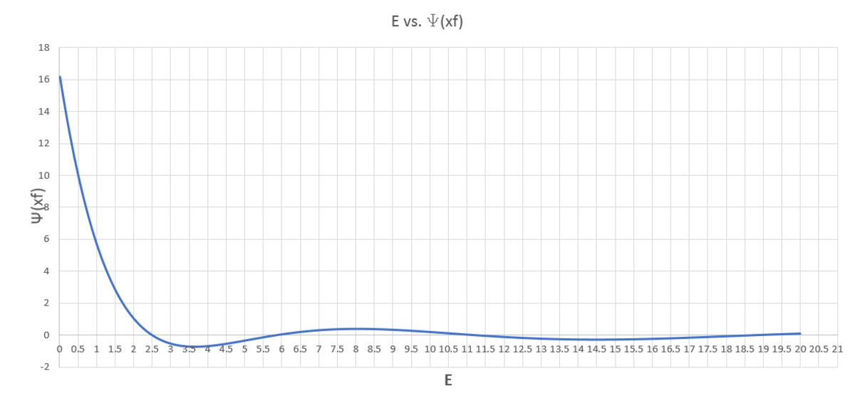
@Karan Chatrath has posted some nice graphs showing the wave function plotted against position for the various allowable energies. I will post a graph of candidate energy levels (swept over a continuum) vs. the value of the corresponding wavefunction at $x = x_f$ . The only allowable values of $E$ are the ones for which the wave function is zero at $x = x_f$ . You can see that $E_2$ is around $6$ (actually $5.848$ ), and $E_3$ is around $11$ (actually $11.25$ ). Simulation code is attached.

import math

xf = 3.0267  # End of well

dE = 10.0/(10.0**3.0)  # Energy increment
dx = xf/(10.0**4.0)    # x increment

E = dE

while E <= 20.0:   # sweep E over a range

    Psi = 0.0      # for every E, initialize Psi and Psi derivative
    Psid = 1.0

    x = 0.0

    V = x
    Psidd = (V-E)*Psi

    ###################################

    while x <= xf:    # for every E, numerically integrate to determine Psi at x = xf

        Psi = Psi + Psid * dx
        Psid = Psid + Psidd * dx

        V = x
        Psidd = (V-E)*Psi

        x = x + dx

    ###################################

    print E,Psi   # Plot E against the value of Psi at x = xf
                  # Allowed energy levels correspond to Psi = 0 at x = xf

    E = E + dE