Cutting random pieces of string
From a string of length 1 m , we choose a length uniformly at random between 0 m and 1 m , and cut as many of these lengths as possible from the string.
What is the expected length of the remaining string (in meters)?
Bonus: If we have a random number a chosen with uniform distribution over the interval ( 0 , n 1 ] , where n ∈ N , what's the expected value of the remainder 1 m o d a for a particular n ?
The answer is 0.1775.
This section requires Javascript.
You are seeing this because something didn't load right. We suggest you, (a) try
refreshing the page, (b) enabling javascript if it is disabled on your browser and,
finally, (c)
loading the
non-javascript version of this page
. We're sorry about the hassle.
5 solutions
This is very nice—you avoid directly computing integrals. This is very desirable.
The first way I solved it was with Matlab (quasi cheating :-). I then went for a walk and came up with a germ of an idea, which turned out to be the same as Zico Quintana's method. I did resort to Wolfram for doing the sum.
Oh my * *! I forgot to multiply by the 1/2;
if i cut the string by 0.6 m , remaining is 0.4m
if i cut it by 0.4 the .4+.4=.8, remaining 0.2m i am not understanding the language of the question
Log in to reply
Umm… you’re computations are correct. You’re not not understanding. Now ‘simply’ compute the ‘average value’ of these remainder lengths.
Log in to reply
why should i do that? i am not understanding the meaning of the question
Log in to reply
@Snehit Panghal – The problem is as follows:
-
For any cutting-length, a ∈ [ 0 , 1 ] , define the ‘remainder length’ as L ( a ) = min { 1 − m a ∣ m > 0 , 1 − m a ≥ 0 } .
-
Now assume a ∼ U ( [ 0 , 1 ] ) ie a is a r.v. uniformly randomly distributed in [ 0 , 1 ] . Compute E [ L ( a ) ] , ie compute the expected (‘average’) value of the remainder lengths.
You already understood 1 fine, as you demonstrated in your computations L ( 0 . 6 ) = 1 − 0 . 6 = 0 . 4 and L ( 0 . 4 ) = 1 − 2 ⋅ 0 . 4 = 0 . 2 . Now do 2. That is what this problem asks.
PS: not ‘I am not understanding’ ⟶ but ‘I don’t understand’. Ing-forms are used to describe what one is doing right now . The former is an unnatural expression.
can somebody explain meaning of the question
I got the process right but I miscalculated it as π^2/12 - 1/2 and hence this is the only question I got wrong this week.
Relevant wiki: Expected Value - Definition
The question is equivalent of asking the expected value of 1 m o d a for random a ∈ ( 0 , 1 ] (why?!).
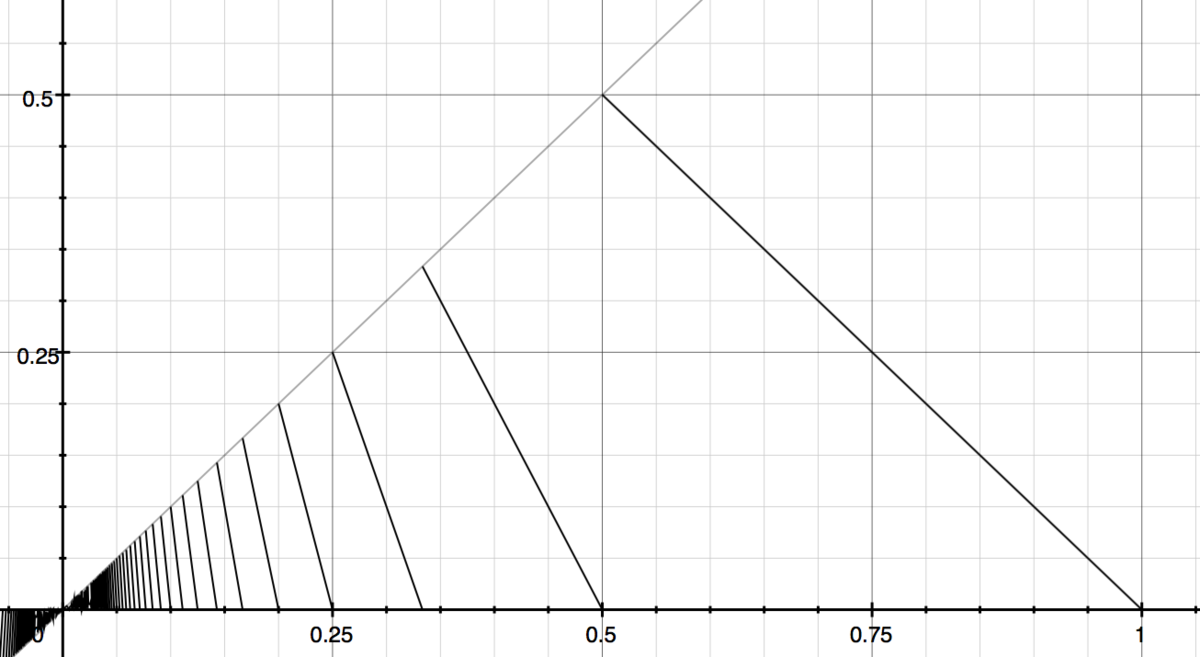
The graph below shows the behavior of
1
m
o
d
x
from 0 to 1, which represents the fraction of the string left when making cuts
x
units long.
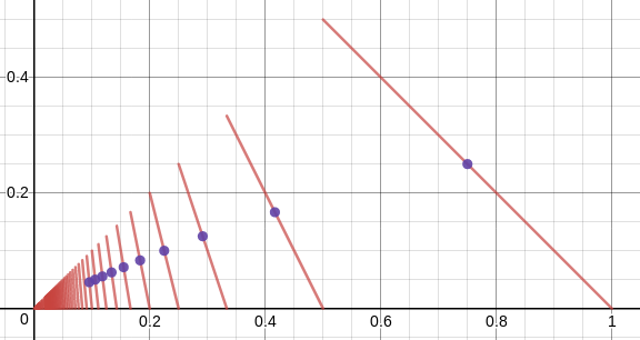 As you can see, you get discontinuities at
n
1
for
n
∈
N
(note that
1
=
n
1
n
+
0
). So we can separate the graph into a series of segments from
(
n
1
,
n
1
)
to
(
n
+
1
1
,
0
)
, starting from n = 1.
As you can see, you get discontinuities at
n
1
for
n
∈
N
(note that
1
=
n
1
n
+
0
). So we can separate the graph into a series of segments from
(
n
1
,
n
1
)
to
(
n
+
1
1
,
0
)
, starting from n = 1.
The n th interval has a leght n 1 − n + 1 1 and an avarage height 2 ( n + 1 ) 1 , so the expected value, which corresponds to the avarage height of the entire function, is equal to the sum of the average heights of the segments weighted by the relative lenght of each interval the segment is contained. As those lenghts add up to 1, the weights are simply the lenghts themselves:
n = 1 ∑ ∞ 2 ( n + 1 ) 1 ( n 1 − n + 1 1 )
This can be rewritten to 2 1 [ n = 1 ∑ ∞ n ( n + 1 ) 1 − n = 1 ∑ ∞ ( n + 1 ) 2 1 ]
The first term is a telescoping series sum that equals 1, and the second term is the sum of the reciprocal of squares minus the first term, which equals ζ ( 2 ) − 1 = 6 π 2 − 1
Thus, the answer is: 2 1 [ 1 − ( 6 π 2 − 1 ) ] 1 − 1 2 π 2 ≈ 0 . 1 7 7 5
Relevant wiki: Expected Value - Problem Solving
Let a denote the r. v. in both problems. Since a is continuously distributed, it is a.e. not of the form n 1 for any n . So a.e. a ∈ ⋃ m ≥ 1 ( m + 1 1 , m 1 ) respectively a ∈ ⋃ m ≥ n ( m + 1 1 , m 1 ) in the second problem.
Let m ∈ N . For a ∈ ( m + 1 1 , m 1 ) it holds that m a < 1 and ( m + 1 ) a > 1 , hence the length a can be cut maximum of m times from 1 leaving L ( a ) = 1 − m a as the remainder. We may thus compute the expected values as follows
[ m ] r c l E [ L ( a ) ∣ a ∈ ( 0 , n 1 ] ] = = = = = = = = = = ∑ m ≥ n P [ a ∈ ( m + 1 1 , m 1 ) ∣ a ∈ ( 0 , n 1 ] ] ⋅ E [ L ( a ) ∣ a ∈ ( m + 1 1 , m 1 ) ] ∑ m ≥ n n 1 − 0 m 1 − m + 1 1 ⋅ E [ 1 − m a ∣ a ∈ ( m + 1 1 , m 1 ) ] ∑ m ≥ n m ( m + 1 ) n ⋅ ( 1 − m E [ a ∣ a ∈ ( m + 1 1 , m 1 ) ] ) ∑ m ≥ n m ( m + 1 ) n ⋅ ( 1 − m ⋅ 2 1 ( m + 1 1 + m 1 ) ) ∑ m ≥ n m ( m + 1 ) n ⋅ ( 1 − 2 ( m + 1 ) 2 m + 1 ) 2 n ∑ m ≥ n m ( m + 1 ) 2 1 2 n ∑ m ≥ n m 1 − m + 1 1 − ( m + 1 ) 2 1 2 n ( n 1 − lim m → ∞ m + 1 1 − ∑ m ≥ n ( m + 1 ) 2 1 ) 2 n ( n 1 − = ζ ( 2 ) = π 2 / 6 m ≥ 1 ∑ m 2 1 + ∑ 1 ≤ m ≤ n m 2 1 ) 2 n ( n 1 + ∑ 1 ≤ m ≤ n m 2 1 − 6 π 2 )
Hence the expected length in the second problem is 2 n ( n 1 + ∑ 1 ≤ m ≤ n m 2 1 − 6 π 2 ) . The first problem is just a special case of this with n = 1 . This yields E [ L ( a ) ] = 2 1 ( 1 + 1 − 6 π 2 ) = 1 − 1 2 π 2 ≈ 0 , 1 7 7 5 3 2 9 6 6 6 .
I did the same, but there's a typo at the end, π^2/6 must be after a minus sing.
Log in to reply
Thanks—typing things up often yields progressive errors when 1 typing mistake occurs—in this case it was generated in the second last line of the longer calculation.
A person with good eyesight should be able to see something .04mm wide (or .0004 metres). It would be sensible to believe the same about length, meaning you can cut 25,000 equal pieces of .04mm rope.
Log in to reply
Are you referring to the a. e. statement? This means, a choice of cuts in { n 1 : n ∈ N + } occurs with probability 0 . It is certainly a possible event, but empirically improbable, as it represents a mere dust of options, compared to the thick range of options of the rest of the unit interval ( 0 , 1 ] .
Log in to reply
No, for the first question as to how long the last piece would be.
Log in to reply
@Joshua Mendez – The questions statement talks about picking a random lenght to cut first, and then making cuts of this lenght until the remaining piece is smaller than this lenght. It's an ideal situation, what do you mean by visual limitations?
@Joshua Mendez – In your example it would be 0 . But your kind of example occurs with probability 0 . If one randomly chooses a length, then almost certainly (with probability 1 ) for any choice the remaining length will be positive. It follows that the average remaining length will be positive.
I plotted the result as y = x % 1.
The y axis is the length of string left, and the x axis represents the starting length. The average length is equal to the integral of this line between 0 and 1. I asked Mr Wolfram, and he didn't give me an answer... 😥
But then I wrote a little JS program to estimate it close enough! 😆
1 2 3 4 5 6 7 |
|
Nice 😃 btw don't you mean y = x % 1 instead of y = x % 3?
Log in to reply
Ooops yep, typo, thanks! Great problem!
Also, I find it really cool how when you go: sqrt(12(1 - 0.17753...)) you get a really nice estimate for pi.
Expected value can be determined using a vast amount of trials. Doing this by hand is not clever, however if you have the patience, go ahead. A simple program in python 3 can bash out the numbers pretty quick and a value that is off by less then 0.0001.
Here is the main gist of the program:
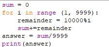
The answer you get is something along the lines of 1774.5759.... Now, since we used 10,000 instead of 1, we need to move the decimal place back 4 places. This turns 1774.5759.. into 0.17745, or roughly 0.1775
Relevant wiki: Discrete Probability Distribution - Uniform Distribution
Let l be the length of the piece(s) being cut, and r the length of the remaining piece.
P [ 2 1 ≤ l ≤ 1 ] = 1 − 2 1 = 2 1 ; and r will be uniformly distributed between 0 and 2 1 , so its expected length will be 4 1
P [ 3 1 ≤ l < 2 1 ] = 2 1 − 3 1 = 6 1 ; and r will be uniformly distributed between 0 and 3 1 , so its expected length will be 6 1
P [ 4 1 ≤ l < 3 1 ] = 3 1 − 4 1 = 1 2 1 ; and r will be uniformly distributed between 0 and 4 1 , so its expected length will be 8 1
⋮
So the expected length of the remaining piece is
( 2 1 ) ( 4 1 ) + ( 6 1 ) ( 6 1 ) + ( 1 2 1 ) ( 8 1 ) + . . . . + ( n ( n + 1 ) 1 ) ( 2 ( n + 1 ) 1 ) + . . . .
The general term can be re-written using partial fractions as
( n ( n + 1 ) 1 ) ( 2 ( n + 1 ) 1 ) = 2 1 ( n ( n + 1 ) 2 1 ) = 2 1 ( n 1 − n + 1 1 − ( n + 1 ) 2 1 )
We can then write the expected length of the remaining piece as
2 1 [ n = 1 ∑ ∞ ( n 1 − n + 1 1 ) − n = 1 ∑ ∞ ( n + 1 ) 2 1 ] = 2 1 [ n = 1 ∑ ∞ ( n 1 − n + 1 1 ) − ( ( n = 1 ∑ ∞ n 2 1 ) − 1 ) ]
The first summation telescopes to 1 ; the second is known as the Basel Problem , which Euler famously found to be 6 π 2 . Thus the expected length of the remaining piece is
2 1 ( 1 − ( 6 π 2 − 1 ) ) = 2 1 ( 2 − 6 π 2 ) = 1 − 1 2 π 2